Data Analysis 2 - Data Wrangling

Learning Objectives

• Describe the purpose of the dplyr package.
• Select certain columns in a data frame with the select function.
• Select certain rows in a data frame according to filtering conditions with the filter function.
• Link the output of one dplyr function to the input of another function with the “pipe” operator %>%.
• Add new columns to a data frame that are functions of existing columns with the mutate function.
• Sort data frames using the arrange() function.
• Use the split-apply-combine concept for data analysis.
• Use summarize, group_by, and count to split a data frame into groups of observations, apply summary statistics for each group, and then combine the results.
• Export a data frame to a .csv file.

Suggested Readings

• Chapter 5 of “R for Data Science”, by Garrett Grolemund and Hadley Wickham
• dplyr cheatsheet

---

R Setup

Before we get started, let’s set up our analysis environment:

1. Open up your “data-analysis-tutorial” R Project that you created in the last lesson - if you didn’t do this, go back and do it now.
2. Create a new .R file (File > New File > R Script), and save it as “data_wrangling.R” inside your “data-analysis-tutorial” R Project folder.
3. Use the download.file() function to download the wildlife_impacts.csv dataset, and save it in the data folder in your R Project:

download.file(
    url = "https://github.com/emse6574-gwu/2019-Fall/raw/gh-pages/data/wildlife_impacts.csv",
    destfile = file.path('data', 'wildlife_impacts.csv')
)

For this lesson, we are going to use the FAA Wildlife Strike Database, which contains records of reported wildlife strikes with aircraft since 1990. Since aircraft-wildlife impacts are voluntarily reported, the database only contains information from airlines, airports, pilots, and other sources and does not represent all strikes. Each row in the dataset holds information for a single strike event with the following columns:

Variable	Class	Description
incident_date	date	Date of incident
state	character	State
airport_id	character	ICAO Airport ID
airport	character	Airport Name
operator	character	Operator/Airline
atype	character	Airline type
type_eng	character	Engine type
species_id	character	Species ID
species	character	Species
damage	character	Damage: N None M Minor, M Uncertain, S Substantial, D Destroyed
num_engs	character	Number of engines
incident_month	double	Incident month
incident_year	double	Incident year
time_of_day	character	Incident Time of day
time	double	Incident time
height	double	Plane height at impact (feet)
speed	double	Plane speed at impact (knots)
phase_of_flt	character	Phase of flight at impact
sky	character	Sky condition
precip	character	Precipitation
cost_repairs_infl_adj	double	Cost of repairs adjusted for inflation

Let’s load our libraries and read in the data:

library(readr)
library(dplyr)
df <- read_csv(file.path('data', 'wildlife_impacts.csv'))

Just like in the last lesson, a good starting point when working with a new dataset is to view some quick summaries. Here’s another summary function (glimpse()) that is similar to str():

glimpse(df)

## Rows: 56,978
## Columns: 21
## $ incident_date         <dttm> 2018-12-31, 2018-12-29, 2018-12-29, 2018-12-27…
## $ state                 <chr> "FL", "IN", "N/A", "N/A", "N/A", "FL", "FL", "N…
## $ airport_id            <chr> "KMIA", "KIND", "ZZZZ", "ZZZZ", "ZZZZ", "KMIA",…
## $ airport               <chr> "MIAMI INTL", "INDIANAPOLIS INTL ARPT", "UNKNOW…
## $ operator              <chr> "AMERICAN AIRLINES", "AMERICAN AIRLINES", "AMER…
## $ atype                 <chr> "B-737-800", "B-737-800", "UNKNOWN", "B-737-900…
## $ type_eng              <chr> "D", "D", NA, "D", "D", "D", "D", "D", "D", "D"…
## $ species_id            <chr> "UNKBL", "R", "R2004", "N5205", "J2139", "UNKB"…
## $ species               <chr> "Unknown bird - large", "Owls", "Short-eared ow…
## $ damage                <chr> "M?", "N", NA, "M?", "M?", "N", "N", "N", "N", …
## $ num_engs              <dbl> 2, 2, NA, 2, 2, 2, 2, 2, 2, 2, 2, 2, 2, 2, 2, 2…
## $ incident_month        <dbl> 12, 12, 12, 12, 12, 12, 12, 12, 12, 12, 12, 12,…
## $ incident_year         <dbl> 2018, 2018, 2018, 2018, 2018, 2018, 2018, 2018,…
## $ time_of_day           <chr> "Day", "Night", NA, NA, NA, "Day", "Night", NA,…
## $ time                  <dbl> 1207, 2355, NA, NA, NA, 955, 948, NA, NA, 1321,…
## $ height                <dbl> 700, 0, NA, NA, NA, NA, 600, NA, NA, 0, NA, 0, …
## $ speed                 <dbl> 200, NA, NA, NA, NA, NA, 145, NA, NA, 130, NA, …
## $ phase_of_flt          <chr> "Climb", "Landing Roll", NA, NA, NA, "Approach"…
## $ sky                   <chr> "Some Cloud", NA, NA, NA, NA, NA, "Some Cloud",…
## $ precip                <chr> "None", NA, NA, NA, NA, NA, "None", NA, NA, "No…
## $ cost_repairs_infl_adj <dbl> NA, NA, NA, NA, NA, NA, NA, NA, NA, NA, NA, NA,…

Wow, there have been 56,978 reported wildlife strikes over the 29 period from 1990 to 2019! On a daily average that comes out to:

nrow(df) / (2019 - 1990) / 365

## [1] 5.3829

…over 5 strikes per day!

Data wrangling with dplyr

[Art by Allison Horst]

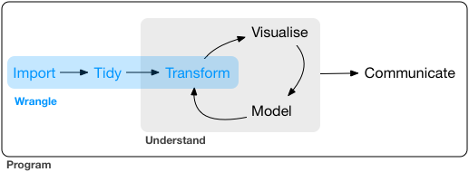
“Data Wrangling” refers to the art of getting your data into R in a useful form for visualization and modeling. Wrangling is the first step in the general data science process:

What is dplyr

As we saw in the last section, we can use brackets ([]) to access elements of a data frame. While this is handy, it can be cumbersome and difficult to read, especially for complicated operations.

Enter dplyr

The dplyr package was designed to make tabular data wrangling easier to perform and read. It pairs nicely with other libraries, such as ggplot2 for visualizing data (which we’ll cover next week). Together, dplyr, ggplot2, and a handful of other packages make up what is known as the “Tidyverse” - an opinionated collection of R packages designed for data science. You can load all of the tidyverse packages at once using the library(tidyverse) command, but for now we’re just going to install and use each package one at a time - starting with dplyr:

install.packages("dplyr")

In this lesson, we are going to learn some of the most common dplyr functions:

• select(): subset columns
• filter(): subset rows on conditions
• mutate(): create new columns by using information from other columns
• arrange(): sort results
• group_by(): group data to perform grouped operations
• summarize(): create summary statistics (usually on grouped data)
• count(): count discrete rows

Select columns with select()

To select specific columns, use select(). The first argument to this function is the data frame (df), and the subsequent arguments are the columns to keep:

# Select only a few columns
select(df, state, damage, time_of_day)

## # A tibble: 56,978 x 3
##    state damage time_of_day
##    <chr> <chr>  <chr>      
##  1 FL    M?     Day        
##  2 IN    N      Night      
##  3 N/A   NA     NA         
##  4 N/A   M?     NA         
##  5 N/A   M?     NA         
##  6 FL    N      Day        
##  7 FL    N      Night      
##  8 N/A   N      NA         
##  9 N/A   N      NA         
## 10 FL    N      Day        
## # … with 56,968 more rows

To select all columns except certain ones, put a - sign in front of the variable to exclude it:

select(df, -state, -damage, -time_of_day)

## # A tibble: 56,978 x 18
##    incident_date       airport_id airport operator atype type_eng species_id
##    <dttm>              <chr>      <chr>   <chr>    <chr> <chr>    <chr>     
##  1 2018-12-31 00:00:00 KMIA       MIAMI … AMERICA… B-73… D        UNKBL     
##  2 2018-12-29 00:00:00 KIND       INDIAN… AMERICA… B-73… D        R         
##  3 2018-12-29 00:00:00 ZZZZ       UNKNOWN AMERICA… UNKN… NA       R2004     
##  4 2018-12-27 00:00:00 ZZZZ       UNKNOWN AMERICA… B-73… D        N5205     
##  5 2018-12-27 00:00:00 ZZZZ       UNKNOWN AMERICA… B-73… D        J2139     
##  6 2018-12-27 00:00:00 KMIA       MIAMI … AMERICA… A-319 D        UNKB      
##  7 2018-12-27 00:00:00 KMCO       ORLAND… AMERICA… A-321 D        UNKBS     
##  8 2018-12-26 00:00:00 ZZZZ       UNKNOWN AMERICA… B-73… D        ZT001     
##  9 2018-12-23 00:00:00 ZZZZ       UNKNOWN AMERICA… A-321 D        ZT101     
## 10 2018-12-23 00:00:00 KFLL       FORT L… AMERICA… B-73… D        I1301     
## # … with 56,968 more rows, and 11 more variables: species <chr>,
## #   num_engs <dbl>, incident_month <dbl>, incident_year <dbl>, time <dbl>,
## #   height <dbl>, speed <dbl>, phase_of_flt <chr>, sky <chr>, precip <chr>,
## #   cost_repairs_infl_adj <dbl>

Some additional options to select columns based on a specific criteria include:

1. ends_with() = Select columns that end with a character string
2. contains() = Select columns that contain a character string
3. matches() = Select columns that match a regular expression
4. one_of() = Select column names that are from a group of names

Select rows with filter()

Filter the rows for wildlife impacts that occurred in DC:

filter(df, state == 'DC')

## # A tibble: 1,228 x 21
##    incident_date       state airport_id airport operator atype type_eng
##    <dttm>              <chr> <chr>      <chr>   <chr>    <chr> <chr>   
##  1 2018-10-23 00:00:00 DC    KDCA       RONALD… AMERICA… B-73… D       
##  2 2018-10-17 00:00:00 DC    KDCA       RONALD… AMERICA… B-73… D       
##  3 2018-10-16 00:00:00 DC    KDCA       RONALD… AMERICA… B-73… D       
##  4 2018-10-12 00:00:00 DC    KDCA       RONALD… AMERICA… B-73… D       
##  5 2018-09-04 00:00:00 DC    KDCA       RONALD… AMERICA… A-319 D       
##  6 2018-09-01 00:00:00 DC    KDCA       RONALD… AMERICA… A-321 D       
##  7 2018-08-31 00:00:00 DC    KIAD       WASHIN… AMERICA… A-319 D       
##  8 2018-08-23 00:00:00 DC    KDCA       RONALD… AMERICA… EMB-… D       
##  9 2018-08-13 00:00:00 DC    KIAD       WASHIN… AMERICA… MD-82 D       
## 10 2018-08-01 00:00:00 DC    KIAD       WASHIN… AMERICA… CRJ7… D       
## # … with 1,218 more rows, and 14 more variables: species_id <chr>,
## #   species <chr>, damage <chr>, num_engs <dbl>, incident_month <dbl>,
## #   incident_year <dbl>, time_of_day <chr>, time <dbl>, height <dbl>,
## #   speed <dbl>, phase_of_flt <chr>, sky <chr>, precip <chr>,
## #   cost_repairs_infl_adj <dbl>

Filter the rows for wildlife impacts that cost more than $1 million in damages:

filter(df, cost_repairs_infl_adj > 10^6)

## # A tibble: 41 x 21
##    incident_date       state airport_id airport operator atype type_eng
##    <dttm>              <chr> <chr>      <chr>   <chr>    <chr> <chr>   
##  1 2015-05-26 00:00:00 N/A   SVMI       SIMON … AMERICA… B-73… D       
##  2 2015-04-25 00:00:00 FL    KJAX       JACKSO… AMERICA… A-319 D       
##  3 2015-04-02 00:00:00 MA    KBOS       GENERA… AMERICA… B-73… D       
##  4 2001-04-02 00:00:00 N/A   LFPG       CHARLE… AMERICA… B-76… D       
##  5 2015-10-08 00:00:00 WA    KSEA       SEATTL… DELTA A… A-330 D       
##  6 2015-09-23 00:00:00 UT    KSLC       SALT L… DELTA A… B-73… D       
##  7 2008-10-25 00:00:00 UT    KSLC       SALT L… DELTA A… DC-9… D       
##  8 2007-12-02 00:00:00 N/A   GOOY       DAKAY-… DELTA A… B-76… D       
##  9 2007-11-22 00:00:00 N/A   LFMN       NICE C… DELTA A… B-76… D       
## 10 2011-07-30 00:00:00 CA    KBUR       BOB HO… SOUTHWE… B-73… D       
## # … with 31 more rows, and 14 more variables: species_id <chr>, species <chr>,
## #   damage <chr>, num_engs <dbl>, incident_month <dbl>, incident_year <dbl>,
## #   time_of_day <chr>, time <dbl>, height <dbl>, speed <dbl>,
## #   phase_of_flt <chr>, sky <chr>, precip <chr>, cost_repairs_infl_adj <dbl>

Sequence operations with pipes (%>%)

(logo is a reference to The Treachery of Images)

What if you want to select and filter at the same time? Well, one way to do this is to use intermediate steps. To do this, you first create a temporary data frame and then use that as input to the next function, like this:

dc_impacts <- filter(df, state == 'DC')
dc_impacts_airlineTime <- select(dc_impacts, operator, time, time_of_day)
head(dc_impacts_airlineTime)

## # A tibble: 6 x 3
##   operator           time time_of_day
##   <chr>             <dbl> <chr>      
## 1 AMERICAN AIRLINES  2130 Night      
## 2 AMERICAN AIRLINES  2043 Night      
## 3 AMERICAN AIRLINES   730 Dawn       
## 4 AMERICAN AIRLINES  2245 Night      
## 5 AMERICAN AIRLINES  2150 Night      
## 6 AMERICAN AIRLINES  2022 Night

This works, but it can also clutter up your workspace with lots of objects with different names.

Another approach is to use pipes, which is a more recent addition to R. Pipes let you take the output of one function and send it directly to the next, which is useful when you need to do many things to the same dataset.

The pipe operator is %>% and comes from the magrittr package, which is installed automatically with dplyr. If you use RStudio, you can type the pipe with Ctrl + Shift + M if you have a PC or Cmd + Shift + M if you have a Mac. Here’s the same thing as the previous example but with pipes:

df %>%
    filter(state == 'DC') %>%
    select(operator, time, time_of_day) %>%
    head()

## # A tibble: 6 x 3
##   operator           time time_of_day
##   <chr>             <dbl> <chr>      
## 1 AMERICAN AIRLINES  2130 Night      
## 2 AMERICAN AIRLINES  2043 Night      
## 3 AMERICAN AIRLINES   730 Dawn       
## 4 AMERICAN AIRLINES  2245 Night      
## 5 AMERICAN AIRLINES  2150 Night      
## 6 AMERICAN AIRLINES  2022 Night

In the above code, we use the pipe to send the df data frame first through filter() to keep only rows from DC, and then through select() to keep only the columns operator, time, and time_of_day.

Since %>% takes the object on its left and passes it as the first argument to the function on its right, we don’t need to explicitly include the data frame as an argument to the filter() and select() functions.

Consider reading the %>% operator as the words “…and then…”. For instance, in the above example I would read the code as “First, filter to only data from DC, and then select the columns operator, time, and time_of_day, and then show the first 6 rows.”

Here’s another analogy:

Without Pipes:

leave_house(get_dressed(get_out_of_bed(wake_up(me))))

With Pipes:

me %>%
    wake_up %>%
    get_out_of_bed %>%
    get_dressed %>%
    leave_house

In the above example, adding pipes makes the flow of operations easier to read from left to right, with the %>% operator reading as “…and then…”

If you want to create a new object with the output of a “pipeline”, you just put the object name at the start of the first pipe:

dc_impacts <- df %>%
    filter(state == 'DC') %>%
    select(operator, time, time_of_day)
head(dc_impacts)

## # A tibble: 6 x 3
##   operator           time time_of_day
##   <chr>             <dbl> <chr>      
## 1 AMERICAN AIRLINES  2130 Night      
## 2 AMERICAN AIRLINES  2043 Night      
## 3 AMERICAN AIRLINES   730 Dawn       
## 4 AMERICAN AIRLINES  2245 Night      
## 5 AMERICAN AIRLINES  2150 Night      
## 6 AMERICAN AIRLINES  2022 Night

Sort rows with arrange()

Use the arrange() function to sort a data frame by a column. For example, if you wanted to view the least expensive accidents, you could arrange the data frame by the variable cost_repairs_infl_adj:

# Arrange by least expensive accident
df %>%
    arrange(cost_repairs_infl_adj)

## # A tibble: 56,978 x 21
##    incident_date       state airport_id airport operator atype type_eng
##    <dttm>              <chr> <chr>      <chr>   <chr>    <chr> <chr>   
##  1 2013-09-05 00:00:00 MI    KFNT       BISHOP… SOUTHWE… B-73… D       
##  2 2011-04-17 00:00:00 TX    KDFW       DALLAS… AMERICA… MD-80 D       
##  3 2018-07-10 00:00:00 NM    KABQ       ALBUQU… SOUTHWE… B-73… D       
##  4 2017-10-31 00:00:00 PA    KPIT       PITTSB… AMERICA… B-73… D       
##  5 2014-01-17 00:00:00 UT    KSLC       SALT L… SOUTHWE… B-73… D       
##  6 2006-04-28 00:00:00 TX    KIAH       GEORGE… UNITED … B-73… D       
##  7 2005-04-13 00:00:00 N/A   ZZZZ       UNKNOWN UNITED … B-76… D       
##  8 2004-06-17 00:00:00 N/A   ZZZZ       UNKNOWN UNITED … B-73… D       
##  9 2004-04-22 00:00:00 N/A   ZZZZ       UNKNOWN UNITED … B-76… D       
## 10 2018-10-20 00:00:00 TX    KDAL       DALLAS… SOUTHWE… B-73… D       
## # … with 56,968 more rows, and 14 more variables: species_id <chr>,
## #   species <chr>, damage <chr>, num_engs <dbl>, incident_month <dbl>,
## #   incident_year <dbl>, time_of_day <chr>, time <dbl>, height <dbl>,
## #   speed <dbl>, phase_of_flt <chr>, sky <chr>, precip <chr>,
## #   cost_repairs_infl_adj <dbl>

To sort in descending order, add the desc() function inside the arrange() function. For example, here are the most expensive accidents:

# Arrange by most expensive accident
df %>%
    arrange(desc(cost_repairs_infl_adj))

## # A tibble: 56,978 x 21
##    incident_date       state airport_id airport operator atype type_eng
##    <dttm>              <chr> <chr>      <chr>   <chr>    <chr> <chr>   
##  1 2009-02-03 00:00:00 CO    KDEN       DENVER… UNITED … B-75… D       
##  2 2007-11-22 00:00:00 N/A   LFMN       NICE C… DELTA A… B-76… D       
##  3 2011-09-26 00:00:00 CO    KDEN       DENVER… UNITED … B-75… D       
##  4 2017-07-11 00:00:00 CO    KDEN       DENVER… UNITED … B-73… D       
##  5 2008-10-25 00:00:00 UT    KSLC       SALT L… DELTA A… DC-9… D       
##  6 2011-07-30 00:00:00 CA    KBUR       BOB HO… SOUTHWE… B-73… D       
##  7 2001-12-06 00:00:00 MI    KDTW       DETROI… SOUTHWE… B-73… D       
##  8 2003-04-15 00:00:00 CA    KSFO       SAN FR… UNITED … B-73… D       
##  9 2005-09-06 00:00:00 CO    KDEN       DENVER… UNITED … B-73… D       
## 10 2005-04-20 00:00:00 N/A   ZZZZ       UNKNOWN UNITED … B-77… D       
## # … with 56,968 more rows, and 14 more variables: species_id <chr>,
## #   species <chr>, damage <chr>, num_engs <dbl>, incident_month <dbl>,
## #   incident_year <dbl>, time_of_day <chr>, time <dbl>, height <dbl>,
## #   speed <dbl>, phase_of_flt <chr>, sky <chr>, precip <chr>,
## #   cost_repairs_infl_adj <dbl>

Create new variables with mutate()

You will often need to create new columns based on the values in existing columns. For this use mutate(). For example, let’s create a new variable converting the height variable from feet to miles:

df %>%
    mutate(height_miles = height / 5280) %>%
    select(height, height_miles)

## # A tibble: 56,978 x 2
##    height height_miles
##     <dbl>        <dbl>
##  1    700        0.133
##  2      0        0    
##  3     NA       NA    
##  4     NA       NA    
##  5     NA       NA    
##  6     NA       NA    
##  7    600        0.114
##  8     NA       NA    
##  9     NA       NA    
## 10      0        0    
## # … with 56,968 more rows

You can also create a second new column based on the first new column within the same call of mutate():

df %>%
    mutate(height_miles = height / 5280,
           height_half_miles = height_miles / 2) %>%
    select(height, height_miles, height_half_miles)

## # A tibble: 56,978 x 3
##    height height_miles height_half_miles
##     <dbl>        <dbl>             <dbl>
##  1    700        0.133            0.0663
##  2      0        0                0     
##  3     NA       NA               NA     
##  4     NA       NA               NA     
##  5     NA       NA               NA     
##  6     NA       NA               NA     
##  7    600        0.114            0.0568
##  8     NA       NA               NA     
##  9     NA       NA               NA     
## 10      0        0                0     
## # … with 56,968 more rows

You’ll notice that the variables created have a lot of NAs - that’s because there are missing data. If you wanted to remove those, you could insert a filter() in the pipe chain:

df %>%
    filter(!is.na(height)) %>%
    mutate(height_miles = height / 5280) %>%
    select(height, height_miles)

## # A tibble: 38,940 x 2
##    height height_miles
##     <dbl>        <dbl>
##  1    700       0.133 
##  2      0       0     
##  3    600       0.114 
##  4      0       0     
##  5      0       0     
##  6      0       0     
##  7    500       0.0947
##  8    100       0.0189
##  9      0       0     
## 10   1000       0.189 
## # … with 38,930 more rows

is.na() is a function that determines whether something is an NA. The ! symbol negates the result, so we’re asking for every row where weight is not an NA.

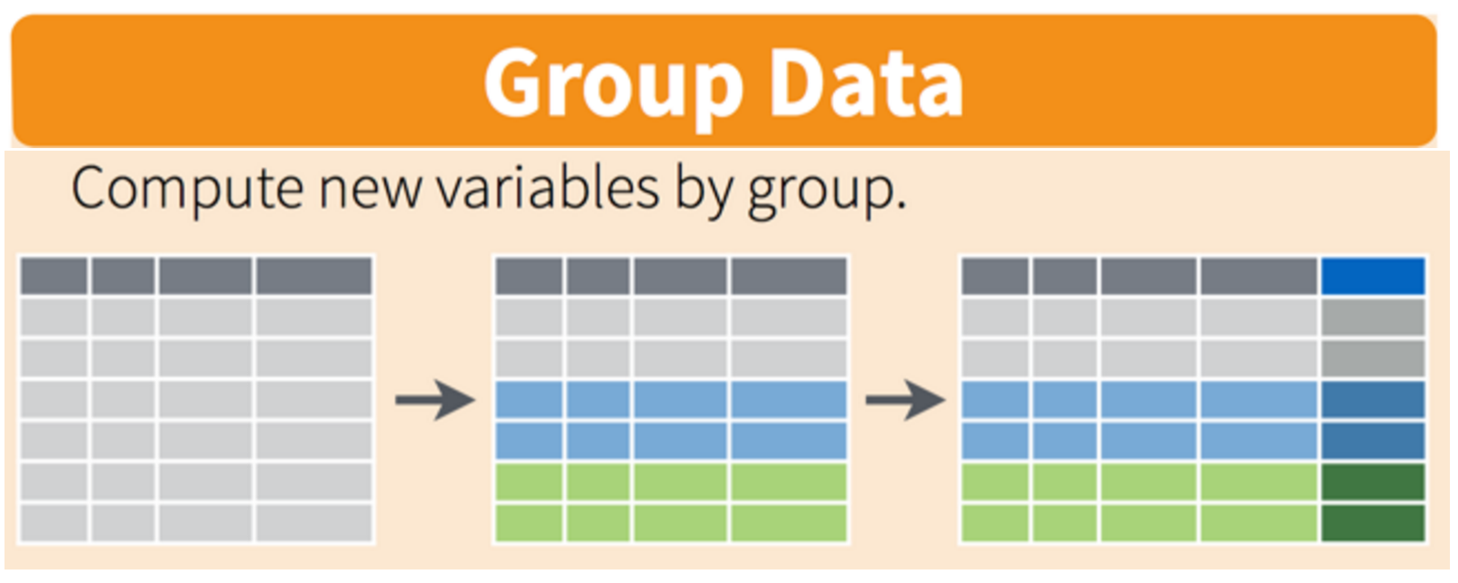
Split-apply-combine

Many data analysis tasks can be approached using the split-apply-combine paradigm:

1. Split the data into groups
2. Apply some analysis to each group
3. Combine the results.

dplyr makes this very easy through the use of the group_by() function.

The group_by() function

The group_by() function enables you to perform operations across groups within the data frame. It is typically used by inserting it in the “pipeline” before the desired group operation. For example, if we wanted to add a a new column that computed the mean height of reported wildlife impacts for each state, we could insert group_by(state) in the pipeline:

df %>%
    filter(!is.na(height)) %>%
    group_by(state) %>%          # Here we're grouping by state
    mutate(mean_height = mean(height)) %>%
    select(state, mean_height)

## # A tibble: 38,940 x 2
## # Groups:   state [59]
##    state mean_height
##    <chr>       <dbl>
##  1 FL           892.
##  2 IN           719.
##  3 FL           892.
##  4 FL           892.
##  5 TX          1177.
##  6 NY           937.
##  7 N/A          994.
##  8 N/A          994.
##  9 MD          1265.
## 10 CA           989.
## # … with 38,930 more rows

You’ll see that the same value for mean_height is reported for the same states (e.g. the mean height in Florida is 892 ft).

The summarize() function

The group_by() function is often used together with summarize(), which collapses each group into a single-row summary of that group. For example, we collapse the result of the previous example by using summarise() instead of mutate():

df %>%
    filter(!is.na(height)) %>%
    group_by(state) %>%
    summarise(mean_height = mean(height))

## `summarise()` ungrouping output (override with `.groups` argument)

## # A tibble: 59 x 2
##    state mean_height
##    <chr>       <dbl>
##  1 AB           327.
##  2 AK           334.
##  3 AL           861.
##  4 AR           968.
##  5 AZ          2134.
##  6 BC           497.
##  7 CA           989.
##  8 CO           442.
##  9 CT           811.
## 10 DC           963.
## # … with 49 more rows

You can also group by multiple columns - here let’s group by state and the airline:

df %>%
    filter(!is.na(height)) %>%
    group_by(state, operator) %>%
    summarise(mean_height = mean(height))

## `summarise()` regrouping output by 'state' (override with `.groups` argument)

## # A tibble: 213 x 3
## # Groups:   state [59]
##    state operator           mean_height
##    <chr> <chr>                    <dbl>
##  1 AB    AMERICAN AIRLINES         318.
##  2 AB    UNITED AIRLINES           350 
##  3 AK    AMERICAN AIRLINES           0 
##  4 AK    DELTA AIR LINES           414.
##  5 AK    UNITED AIRLINES           311.
##  6 AL    AMERICAN AIRLINES        1038.
##  7 AL    DELTA AIR LINES           485.
##  8 AL    SOUTHWEST AIRLINES       1020.
##  9 AL    UNITED AIRLINES           375 
## 10 AR    AMERICAN AIRLINES         508.
## # … with 203 more rows

Notice that in the above examples I’ve kept the early filter to drop NAs. This is important when performing summarizing functions like mean() or sum(). If NAs are present, the result will also be NA:

df %>%
    group_by(state) %>%
    summarise(mean_height = mean(height))

## `summarise()` ungrouping output (override with `.groups` argument)

## # A tibble: 59 x 2
##    state mean_height
##    <chr>       <dbl>
##  1 AB            NA 
##  2 AK           334.
##  3 AL            NA 
##  4 AR            NA 
##  5 AZ            NA 
##  6 BC            NA 
##  7 CA            NA 
##  8 CO            NA 
##  9 CT            NA 
## 10 DC            NA 
## # … with 49 more rows

Once the data are grouped, you can also summarize multiple variables at the same time (and not necessarily on the same variable). For instance, you could add two more columns computing the minimum and maximum height:

df %>%
    filter(!is.na(height)) %>%
    group_by(state, operator) %>%
    summarise(mean_height = mean(height),
              min_height = min(height),
              max_height = max(height))

## `summarise()` regrouping output by 'state' (override with `.groups` argument)

## # A tibble: 213 x 5
## # Groups:   state [59]
##    state operator           mean_height min_height max_height
##    <chr> <chr>                    <dbl>      <dbl>      <dbl>
##  1 AB    AMERICAN AIRLINES         318.          0       1300
##  2 AB    UNITED AIRLINES           350           0       1400
##  3 AK    AMERICAN AIRLINES           0           0          0
##  4 AK    DELTA AIR LINES           414.          0       1700
##  5 AK    UNITED AIRLINES           311.          0       1200
##  6 AL    AMERICAN AIRLINES        1038.          0      11300
##  7 AL    DELTA AIR LINES           485.          0       5400
##  8 AL    SOUTHWEST AIRLINES       1020.          0      10000
##  9 AL    UNITED AIRLINES           375           0       2800
## 10 AR    AMERICAN AIRLINES         508.          0       3400
## # … with 203 more rows

Counting

Often times you will want to know the number of observations found for each variable or combination of variables. One way to do this is to use the group_by() and summarise() functions in combination. For example, here is the number of observations for each aircraft engine type:

df %>%
    group_by(type_eng) %>%
    summarise(count = n())

## `summarise()` ungrouping output (override with `.groups` argument)

## # A tibble: 5 x 2
##   type_eng count
##   <chr>    <int>
## 1 A            2
## 2 C           34
## 3 D        56705
## 4 F            3
## 5 NA         234

Since this is such a common task, dplyr provides the count() function to do the same thing:

df %>%
    count(type_eng)

## # A tibble: 5 x 2
##   type_eng     n
##   <chr>    <int>
## 1 A            2
## 2 C           34
## 3 D        56705
## 4 F            3
## 5 NA         234

For convenience, count() also provides the sort argument:

df %>%
    count(type_eng, sort = TRUE)

## # A tibble: 5 x 2
##   type_eng     n
##   <chr>    <int>
## 1 D        56705
## 2 NA         234
## 3 C           34
## 4 F            3
## 5 A            2

You can also count the combination of variables by providing more than one column name to count():

df %>%
    count(type_eng, num_engs, sort = TRUE)

## # A tibble: 10 x 3
##    type_eng num_engs     n
##    <chr>       <dbl> <int>
##  1 D               2 53652
##  2 D               3  2753
##  3 D               4   299
##  4 NA             NA   232
##  5 C               2    34
##  6 F               2     3
##  7 NA              2     2
##  8 A               1     1
##  9 A               2     1
## 10 D              NA     1

Hmm, looks like most reported wildlife impacts involve planes with 2 D-type engines.

Exporting data

Now that you have learned how to use dplyr to extract information from or summarize your raw data, you may want to export these new data sets. Similar to the read_csv() function used for reading CSV files into R, there is a write_csv() function that generates CSV files from data frames.

Important: Before using write_csv(), create a new folder called “data_output” and put it in your R Project folder. In general, you should never write generated datasets in the same directory as your raw data. The “data” folder should only contain the raw, unaltered data, and should be left alone to make sure we don’t delete or modify it.

Let’s save one of the summary data frames from the earlier examples where we computed the min, mean, and max heights of impacts by each state and airline:

heightSummary <- df %>%
    filter(!is.na(height)) %>%
    group_by(state, operator) %>%
    summarise(mean_height = mean(height),
              min_height = min(height),
              max_height = max(height))

## `summarise()` regrouping output by 'state' (override with `.groups` argument)

Save the the new heightSummary data frame as a CSV file in your “data_output” folder:

write_csv(heightSummary, path = file.path('data_output', 'heightSummary.csv')

---

Tips

You will often need to create new variables based on a condition. To do this, you can use the if_else() function. Here’s the general syntax:

if_else(<condition>, <if TRUE>, <else>)

The first argument is a condition. If the condition is TRUE, then the value given to the second argument will be used; if not, then the third argument value will be used.

Here’s an example of creating a variable to determine which months in the wildlife impacts data are in the summer:

df %>%
    mutate(
        summer_month = if_else(incident_month %in% c(6, 7, 8), TRUE, FALSE))

Of course, in this particular case the if_else() function isn’t even needed because the condition returns TRUE and FALSE values. However, if you wanted to extend this example to determine all four seasons, you could use a series of nested if_else() functions:

df %>%
    mutate(season =
        if_else(
            incident_month %in% c(3, 4, 5), 'Spring',
        if_else(
            incident_month %in% c(6, 7, 8), 'Summer',
        if_else(
            incident_month %in% c(9, 10, 11), 'Fall', 'Winter'))))

Note: The Base R version of this function is ifelse(), but I recommend using the dplyr version, if_else(), as it is a stricter function.

---

Page sources:

Some content on this page has been modified from other courses, including:

• Data Analysis and Visualization in R for Ecologists, by François Michonneau & Auriel Fournier. Zenodo: http://doi.org/10.5281/zenodo.3264888
• The amazing illustrations by Allison Horst

---

EMSE 4574: Programming for Analytics (Fall 2020) |
Tuesdays | 12:45 - 3:15 PM | Dr. John Paul Helveston | jph@gwu.edu
Content 2020 John Paul Helveston. See the licensing page for details.