Learning Objectives

Know some common functions in R.

Know how R handles function arguments and named arguments.

Know how to install, load, and use functions from external R packages.

Practice programming with functions using the TurtleGraphics package.

Suggested Readings

Chapter 3.5 of Danielle Navarro’s book “Learning Statistics With R”

Functions

You can do a lot with the basic operators like +, -, and *, but to do more advanced calculations you’re going to need to start using functions.¹

Watch this 1-minute video for a quick summary of functions

R has a lot of very useful built-in functions. For example, if I wanted to take the square root of 225, I could use R’s built-in square root function sqrt():

sqrt(225)

## [1] 15

Here the letters sqrt are short for “square root,” and the value inside the () is the “argument” to the function. In the example above, the value 225 is the “argument”.

Keep in mind that not all functions have (or require) arguments:

date() # Returns the current date and time

## [1] "Tue Dec 15 17:50:42 2020"

(the date above is the date this page was last built)

Multiple arguments

Some functions have more than one argument. For example, the round() function can be used to round some value to the nearest integer or to a specified decimal place:

round(3.14165)    # Rounds to the nearest integer

## [1] 3

round(3.14165, 2) # Rounds to the 2nd decimal place

## [1] 3.14

Not all arguments are mandatory. With the round() function, the decimal place is an optional input - if nothing is provided, the function will round to the nearest integer by default.

Argument names

In the case of round(), it’s not too hard to remember which argument comes first and which one comes second. But it starts to get very difficult once you start using complicated functions that have lots of arguments. Fortunately, most R functions use argument names to make your life a little easier. For the round() function, for example, the number that needs to be rounded is specified using the x argument, and the number of decimal points that you want it rounded to is specified using the digits argument, like this:

round(x = 3.1415, digits = 2)

## [1] 3.14

Default values

Notice that the first time I called the round() function I didn’t actually specify the digits argument at all, and yet R somehow knew that this meant it should round to the nearest whole number. How did that happen? The answer is that the digits argument has a default value of 0, meaning that if you decide not to specify a value for digits then R will act as if you had typed digits = 0.

This is quite handy: most of the time when you want to round a number you want to round it to the nearest whole number, and it would be pretty annoying to have to specify the digits argument every single time. On the other hand, sometimes you actually do want to round to something other than the nearest whole number, and it would be even more annoying if R didn’t allow this! Thus, by having digits = 0 as the default value, we get the best of both worlds.

Function help

Not sure what a function does, how many arguments it has, or what the argument names are? Ask R for help by typing ? and then the function name, and R will return some documentation about it. For example, type ?round() into the console and R will return information about how to use the round() function.

Combining functions

In the same way that R allows us to put multiple operations together into a longer command (like 1 + 2 * 4 for instance), it also lets us put functions together and even combine functions with operators if we so desire. For example, the following is a perfectly legitimate command:

round(sqrt(7), digits = 2)

## [1] 2.65

When R executes this command, starts out by calculating the value of sqrt(7), which produces an intermediate value of 2.645751. The command then simplifies to round(2.645751, digits = 2), which rounds the value to 2.65.

Frequently used functions

Math functions

R has LOTS of functions. Many of the basic math functions are somewhat self-explanatory, but it can be hard to remember the specific function name. Below is a reference table of some frequently used math functions.

Function	Description	Example input	Example output
`round(x, digits=0)`	Round `x` to the `digits` decimal place	`round(3.1415, digits=2)`	`3.14`
`floor(x)`	Round `x` down the nearest integer	`floor(3.1415)`	`3`
`ceiling(x)`	Round `x` up the nearest integer	`ceiling(3.1415)`	`4`
`abs()`	Absolute value	`abs(-42)`	`42`
`min()`	Minimum value	`min(1, 2, 3)`	`1`
`max()`	Maximum value	`max(1, 2, 3)`	`3`
`sqrt()`	Square root	`sqrt(64)`	`8`
`exp()`	Exponential	`exp(0)`	`1`
`log()`	Natural log	`log(1)`	`0`
`factorial()`	Factorial	`factorial(5)`	`120`

Functions for manipulating data types

You will often need to check the data type of objects and convert them to other types. To handle this, use these patterns:

Check the type of x: is.______()
Convert the type of x: as.______()

In each of these patterns, replace “______” with:

character
logical
numeric / double / integer

Converting data types

You can convert an object from one type to another using as.______(), replacing “______” with a data type:

Convert numeric types:

as.numeric("3.1415")

## [1] 3.1415

as.double("3.1415")

## [1] 3.1415

as.integer("3.1415")

## [1] 3

Convert non-numeric types:

as.character(3.1415)

## [1] "3.1415"

as.logical(3.1415)

## [1] TRUE

A few notes to keep in mind:

When converting from a numeric to a logical, as.logical() will always return TRUE for any numeric value other than 0, for which it returns FALSE.
```
as.logical(7)
```
```
## [1] TRUE
```
```
as.logical(0)
```
```
## [1] FALSE
```
The reverse is also true
```
as.numeric(TRUE)
```
```
## [1] 1
```
```
as.numeric(FALSE)
```
```
## [1] 0
```
Not everything can be converted. For example, if you try to coerce a character that contains letters into a number, R will return NA, because it doesn’t know what number to choose:
```
as.numeric('foo')
```
```
## Warning: NAs introduced by coercion
```
```
## [1] NA
```
The as.integer() function behaves the same as floor():
```
as.integer(3.14)
```
```
## [1] 3
```
```
as.integer(3.99)
```
```
## [1] 3
```

Checking data types

Similar to the as.______() format, you can check if an object is a specific data type using is.______(), replacing “______” with a data type.

Checking numeric types:

is.numeric(3.1415)

## [1] TRUE

is.double(3.1415)

## [1] TRUE

is.integer(3.1415)

## [1] FALSE

Checking non-numeric types:

is.character(3.1415)

## [1] FALSE

is.logical(3.1415)

## [1] FALSE

One thing you’ll notice is that is.integer() often gives you a surprising result. For example, why did is.integer(7) return FALSE?. Well, this is because numbers are doubles by default in R, so even though 7 looks like an integer, R thinks it’s a double.

The safer way to check if a number is an integer in value is to compare it against itself converted into an integer:

7 == as.integer(7)

## [1] TRUE

More functions with packages

When you start R, it only loads the “Base R” functions (e.g. sqrt(), round(), etc.), but there are thousands and thousands of additional functions stored in external packages.

Watch this 1-minute video for a quick summary of packages

Installing packages

To install a package, use the install.packages() function. Make sure you put the package name in quotes:

install.packages("packagename") # This works
install.packages(packagename)   # This doesn't work

Just like most software, you only need to install a package once.

Using packages

After installing a package, you can’t immediately use the functions that the package contains. This is because when you start up R only the “base” functions are loaded. If you want R to also load the functions inside a package, you have to load that package, which you do with the library() function. In contrast to the install.packages() function, you don’t need quotes around the package name to load it:

library("packagename") # This works
library(packagename)   # This also works

Here’s a helpful image to keep the two ideas of installing vs loading separate:

Example: wikifacts

As an example, try installing the Wikifacts package, by Keith McNulty:

install.packages("wikifacts") # Remember - you only have to do this once!

Now that you have the package installed on your computer, try loading it using library(wikifacts), then trying using some of it’s functions:

library(wikifacts) # Load the library

wiki_randomfact()

## [1] "Did you know that before his death at the Battle of Barnet in 1471, John Neville was reported to be in the thick of the fighting and \"cutting off arms and heads like a hero of romance\"? (Courtesy of Wikipedia)"

wiki_didyouknow()

## [1] "Did you know that the Federal Radio Commission revoked the license of Chicago radio station WCHI in 1931 for attacking medical procedures such as surgical operations and vaccinations? (Courtesy of Wikipedia)"

In case you’re wondering, the only thing this package does is generate messages containing random facts from Wikipedia.

Using only some package functions

Sometimes you may only want to use a single function from a library without having to load the whole thing. To do so, use this recipe:

packagename::functionname()

Here I use the name of the package followed by :: to tell R that I’m looking for a function that is in that package. For example, if I didn’t want to load the whole wikifacts library but still wanted to use the wiki_randomfact() function, I could do this:

wikifacts::wiki_randomfact()

## [1] "Did you know that Mamamoo's Melting was described as \"heralding the Korean quartet's rise to the top ranks of the girl group hunger games\"? (Courtesy of Wikipedia)"

Where this is particularly handy is when two packages have a function with the same name. If you load both library, R might not know which function to use. In those cases, it’s best to also provide the package name. For example, let’s say there was a package called apples and another called bananas, and each had a function named fruitName(). If I wanted to use each of them in my code, I would need to specify the package names like this:

apples::fruitName()
bananas::fruitName()

Turtle Graphics

Turtle graphics is a classic teaching tool in computer science, originally invented in the 1960s and re-implemented over and over again in different programming languages.

In R, there is a similar package called TurtleGraphics. To get started, install the package (remember, you only need to do this once on your computer):

install.packages('TurtleGraphics')

Once installed, load the package (remember, you have to load this every time you restart R to use the package!):

library(TurtleGraphics)

## Loading required package: grid

Getting to know your turtle

Here’s the idea. You have a turtle, and she lives in a nice warm terrarium. The terrarium is 100 x 100 units in size, where the lower-left corner is at the (x, y) position of (0, 0). When you call turtle_init(), the turtle is initially positioned in the center of the terrarium at (50, 50):

turtle_init()

You can move the turtle using a variety of movement functions (see ?turtle_move()), and she will leave a trail where ever she goes. For example, you can move her 10 units forward from her starting position:

turtle_init()
turtle_forward(distance = 10)

You can also make the turtle jump to a new position (without drawing a line) by using the turtle_setpos(x, y), where (x, y) is a coordinate within the 100 x 100 terrarium:

turtle_init()
turtle_setpos(x=10, y=10)

Turtle loops

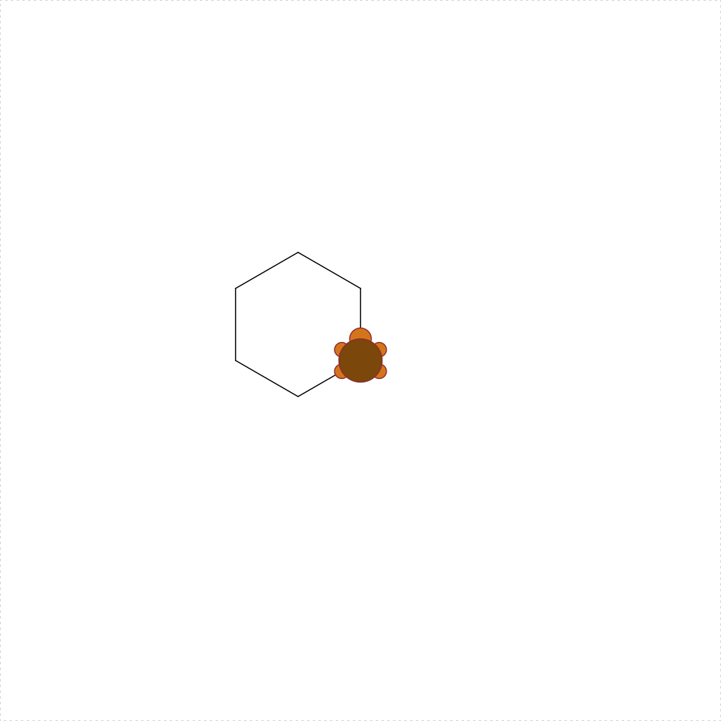
Simple enough, right? But what if I want my turtle to draw a more complicated shape? Let’s say I want her to draw a hexagon. There are six sides to the hexagon, so the most natural way to write code for this is to write a for loop that loops over the sides (don’t worry if this doesn’t make sense yet - we’ll get to loops in week 5!). At each iteration within the loop, I’ll have the turtle walk forwards, and then turn 60 degrees to the left. Here’s what happens:

turtle_init()
for (side in 1:6) {
    turtle_forward(distance = 10)
    turtle_left(angle = 60)
}

Cool! As you draw more complex shapes, you can speed up the process by wrapping your turtle commands inside the turtle_do({}) function. This will skip the animations of the turtle moving and will jump straight to the final position. For example, here’s the hexagon again without animations:

turtle_init()
turtle_do({
    for (side in 1:6) {
        turtle_forward(distance = 10)
        turtle_left(angle = 60)
    }
})

Page sources:

Some content on this page has been modified from other courses, including:

Danielle Navarro’s book “Learning Statistics With R”
Danielle Navarro’s website “R for Psychological Science”
Jenny Bryan’s STAT 545 Course
RStudio primers
Xiao Ping Song’s Intro2R crash course

Technically speaking, operators are functions in R: the addition operator + is a convenient way of calling the addition function '+'(). Thus 10+20 is equivalent to the function call '+'(20, 30). Not surprisingly, no-one ever uses this version.↩︎

EMSE 4574: Programming for Analytics (Fall 2020) |
Tuesdays | 12:45 - 3:15 PM | Dr. John Paul Helveston | jph@gwu.edu
Content 2020 John Paul Helveston. See the licensing page for details.

Functions & Packages

Learning Objectives

Suggested Readings