Data Analysis 1 - Data Frames
This is the first lesson in a sequence on data analysis in R. Before reading this lesson, check out the “Prelude to Data Analysis”.
Learning Objectives
- Describe what a data frame is.
- Create data frames.
- Use indexing to subset and modify specific portions of data frames.
- Load external data from a .csv file into a data frame.
- Summarize the contents of a data frame.
Suggested Readings
- “Introduction to Data frames in R” Data Camp article, by Ryan Sheehy
- Chapter 10 of “R for Data Science”, by Garrett Grolemund and Hadley Wickham
- Chapters 5.8 - 5.11 of “Hands-On Programming with R”, by Garrett Grolemund
1 The data frame
1.1 What are data frames?
Data frames are the de facto data structure for most tabular
data in R. A data frame can be created by hand, but most commonly they
are generated by reading in a data file (typically a .csv
file).
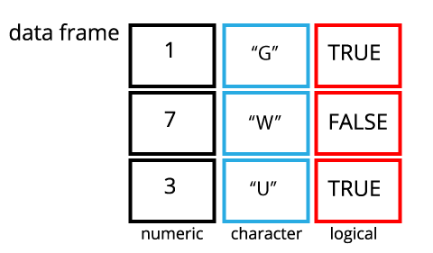
A data frame is the representation of data in the format of a table where the columns are vectors of the same length. Because columns are vectors, each column must contain a single type of data (e.g., numeric, character, integer, logical). For example, here is a figure depicting a data frame comprising a numeric, a character, and a logical vector:
1.2 The
data.frame() function
You can create a data frame using the data.frame()
function. Here is an example using of members of the Beatles band:
beatles <- data.frame(
    firstName   = c("John", "Paul", "Ringo", "George"),
    lastName    = c("Lennon", "McCartney", "Starr", "Harrison"),
    instrument  = c("guitar", "bass", "drums", "guitar"),
    yearOfBirth = c(1940, 1942, 1940, 1943),
    deceased    = c(TRUE, FALSE, FALSE, TRUE)
)
beatles
## firstName lastName instrument yearOfBirth deceased
## 1 John Lennon guitar 1940 TRUE
## 2 Paul McCartney bass 1942 FALSE
## 3 Ringo Starr drums 1940 FALSE
## 4 George Harrison guitar 1943 TRUENotice how the data frame is created - you just hand the
data.frame() function a bunch of vectors! This should
hopefully help make it clear that a data frame is indeed a series of
same-length vectors structured side-by-side.
1.3 The
tibble() function
The tibble is an improved version of the Base R data frame, and it comes from the dplyr library (which we’ll get into next lesson). If you haven’t already, go ahead and install and load the dplyr library now:
install.packages('dplyr')
library(dplyr)
A tibble works just like a data frame, but it has a few small features that make it a bit more useful - to the extent that from here on, we will be using tibbles as our default data frame structure. With this in mind, I’ll often use the term “data frame” to refer to both tibbles and data frames, since they serve the same purpose as a data structure.
Just like with data frames, you can create a tibble using the
tibble() function. Here’s the same example as before with
the Beatles band:
beatles <- tibble(
    firstName   = c("John", "Paul", "Ringo", "George"),
    lastName    = c("Lennon", "McCartney", "Starr", "Harrison"),
    instrument  = c("guitar", "bass", "drums", "guitar"),
    yearOfBirth = c(1940, 1942, 1940, 1943),
    deceased    = c(TRUE, FALSE, FALSE, TRUE)
)
beatles
## # A tibble: 4 × 5
## firstName lastName instrument yearOfBirth deceased
## <chr> <chr> <chr> <dbl> <lgl>
## 1 John Lennon guitar 1940 TRUE
## 2 Paul McCartney bass 1942 FALSE
## 3 Ringo Starr drums 1940 FALSE
## 4 George Harrison guitar 1943 TRUEHere we can see a couple of the differences that make tibbles a bit more intuitive to use:
- It’s easier to see what type of data each column is because tibbles
display this in between the
<>symbols under each column name. - A tibble will only print the first few rows of data when you enter the object name. In contrast, data frames will try to print the entire data frame (which is super annoying when you have a data frame with millions of rows of data). Here, we only have 4 rows, so this difference is not apparent.
- Columns of class
characterare never converted into factors (don’t worry about this for now…just know that keeping strings as acharacterclass generally makes life easier in R).
Now that we have a data frame (tibble) defined, let’s see what we can do with it!
1.4 Dimensions
You can get the dimensions of a data frame using the
ncol(), nrow(), and dim()
functions:
nrow(beatles) # Returns the number of rows## [1] 4ncol(beatles) # Returns the number of columns## [1] 5dim(beatles) # Returns a vector of the number rows and columns## [1] 4 51.5 Row and column names
Data frames must have column names, but row names
are optional (by default, row names are just a sequence of numbers). The
names() function returns the column names, or you can also
be more specific and use the colnames() and
rownames() functions:
names(beatles) # Returns a vector of the column names## [1] "firstName" "lastName" "instrument" "yearOfBirth" "deceased"colnames(beatles) # Also returns a vector of the column names## [1] "firstName" "lastName" "instrument" "yearOfBirth" "deceased"rownames(beatles) # Returns a vector of the row names## [1] "1" "2" "3" "4"1.6 Combining data frames
You can combine data frames using the bind_cols() and
bind_rows() functions:
# Combine columns
names <- tibble(
    firstName = c("John", "Paul", "Ringo", "George"),
    lastName  = c("Lennon", "McCartney", "Starr", "Harrison")
)
instruments <- tibble(
    instrument = c("guitar", "bass", "drums", "guitar")
)
bind_cols(names, instruments)
## # A tibble: 4 × 3
## firstName lastName instrument
## <chr> <chr> <chr>
## 1 John Lennon guitar
## 2 Paul McCartney bass
## 3 Ringo Starr drums
## 4 George Harrison guitar# Combine rows
members1 <- tibble(
firstName = c("John", "Paul"),
lastName = c("Lennon", "McCartney")
)
members2 <- tibble(
firstName = c("Ringo", "George"),
lastName = c("Starr", "Harrison")
)
bind_rows(members1, members2)## # A tibble: 4 × 2
## firstName lastName
## <chr> <chr>
## 1 John Lennon
## 2 Paul McCartney
## 3 Ringo Starr
## 4 George HarrisonNote that to combine rows, the column names must be the same. For
example, if we change the second column name in members2 to
"LASTNAME", you’ll get a data frame with three columns, two
of which will have missing values:
colnames(members2) <- c("firstName", "LASTNAME")
bind_rows(members1, members2)
## # A tibble: 4 × 3
## firstName lastName LASTNAME
## <chr> <chr> <chr>
## 1 John Lennon <NA>
## 2 Paul McCartney <NA>
## 3 Ringo <NA> Starr
## 4 George <NA> Harrison2 Accessing elements
2.1 Using the
$ operator
You can extract columns from a data frame by name by using the
$ operator plus the column name. For example, the
instrument column can be accessed using
beatles$instrument:
beatles$instrument## [1] "guitar" "bass" "drums" "guitar"2.2 Using integer indices
You can access elements in a data frame using brackets
[] and indices inside the brackets. The general form
is:
DF[ROWS, COLUMNS]To index with integers, specify the row numbers and column numbers as vectors.
beatles[1, 2] # Select the element in row 1, column 2## # A tibble: 1 × 1
## lastName
## <chr>
## 1 Lennonbeatles[c(1, 2), c(2, 3)] # Select the elements in rows 1 & 2 and columns 2 & 3## # A tibble: 2 × 2
## lastName instrument
## <chr> <chr>
## 1 Lennon guitar
## 2 McCartney bassbeatles[1:2, 2:3] # Same thing, but using the ":" operator## # A tibble: 2 × 2
## lastName instrument
## <chr> <chr>
## 1 Lennon guitar
## 2 McCartney bassIf you leave either the row or column index blank, it means “selects all”:
beatles[c(1, 2),] # Leaving the column index blank will select all columns## # A tibble: 2 × 5
## firstName lastName instrument yearOfBirth deceased
## <chr> <chr> <chr> <dbl> <lgl>
## 1 John Lennon guitar 1940 TRUE
## 2 Paul McCartney bass 1942 FALSEbeatles[,c(1, 2)] # Leaving the row index blank will select all rows## # A tibble: 4 × 2
## firstName lastName
## <chr> <chr>
## 1 John Lennon
## 2 Paul McCartney
## 3 Ringo Starr
## 4 George HarrisonYou can also use negative integers to specify rows or columns to be excluded:
beatles[-1, ] # Select all rows and except the first## # A tibble: 3 × 5
## firstName lastName instrument yearOfBirth deceased
## <chr> <chr> <chr> <dbl> <lgl>
## 1 Paul McCartney bass 1942 FALSE
## 2 Ringo Starr drums 1940 FALSE
## 3 George Harrison guitar 1943 TRUE2.3 Using character indices
You can use the column names to select elements in a data frame. If
you do not include a , to designate which rows to select, R
will return all the rows for the selected columns:
beatles[c('firstName', 'lastName')] # Select all rows for the "firstName" and "lastName" columns## # A tibble: 4 × 2
## firstName lastName
## <chr> <chr>
## 1 John Lennon
## 2 Paul McCartney
## 3 Ringo Starr
## 4 George Harrisonbeatles[1:2, c('firstName', 'lastName')] # Select just the first two rows for the "firstName" and "lastName" columns## # A tibble: 2 × 2
## firstName lastName
## <chr> <chr>
## 1 John Lennon
## 2 Paul McCartney2.4 Using logical indices
When using a logical vector for indexing, the position where the
logical vector is TRUE is returned. This is helpful for
filtering data frame rows based on conditions. For example, if you
wanted to filter out the rows for which Beatles members were still
alive, you could first create a logical vector using the
deceased column:
beatles$deceased == FALSE## [1] FALSE TRUE TRUE FALSEThen, you could insert this logical vector in the row position of the
[] brackets to filter only the rows that are
TRUE:
beatles[beatles$deceased == FALSE,]## # A tibble: 2 × 5
## firstName lastName instrument yearOfBirth deceased
## <chr> <chr> <chr> <dbl> <lgl>
## 1 Paul McCartney bass 1942 FALSE
## 2 Ringo Starr drums 1940 FALSE2.5 Modifying data frames
You can use any of the above methods for accessing elements in a data
frame to also modify those elements using the assignment operator
(<-). In addition to using brackets to modify specific
elements, you can use the $ operator to create new columns
in a data frame.
For example, let’s create the variable age by
subtracting the yearOfBirth variable from the current
year:
beatles$age <- 2019 - beatles$yearOfBirth
beatles
## # A tibble: 4 × 6
## firstName lastName instrument yearOfBirth deceased age
## <chr> <chr> <chr> <dbl> <lgl> <dbl>
## 1 John Lennon guitar 1940 TRUE 79
## 2 Paul McCartney bass 1942 FALSE 77
## 3 Ringo Starr drums 1940 FALSE 79
## 4 George Harrison guitar 1943 TRUE 76You can also make a new column of all the same value by just providing one value:
beatles$hometown <- 'Liverpool'
beatles
## # A tibble: 4 × 7
## firstName lastName instrument yearOfBirth deceased age hometown
## <chr> <chr> <chr> <dbl> <lgl> <dbl> <chr>
## 1 John Lennon guitar 1940 TRUE 79 Liverpool
## 2 Paul McCartney bass 1942 FALSE 77 Liverpool
## 3 Ringo Starr drums 1940 FALSE 79 Liverpool
## 4 George Harrison guitar 1943 TRUE 76 Liverpool3 Dealing with actual data
Now that we know what a data frame is, let’s start working with
actual data! We are going to use the msleep dataset, which
contains data on sleep times and weights of different mammals. The data
are taken from V.
M. Savage and G. B. West. “A quantitative, theoretical framework for
understanding mammalian sleep.” Proceedings of the National Academy
of Sciences, 104 (3):1051-1056, 2007..
The dataset is stored as a comma separated value (CSV) file. Each row holds information for a single animal, and the columns represent:
| Column Name | Description |
|---|---|
| name | Common name |
| genus | The taxonomic genus of animal |
| vore | Carnivore, omnivore or herbivore? |
| order | The taxonomic order of animal |
| conservation | The conservation status of the animal |
| sleep_total | Total amount of sleep, in hours |
| sleep_rem | REM sleep, in hours |
| sleep_cycle | Length of sleep cycle, in hours |
| awake | Amount of time spent awake, in hours |
| brainwt | Brain weight in kilograms |
| bodywt | Body weight in kilograms |
3.1 R Setup
Before we dig into the data, let’s prepare our analysis environment by following these steps:
- Create a new R Project called “data-analysis-tutorial” and save the folder somewhere on your computer (see the “RStudio projects” section from waaaaay back on week 1).
- Create a new
.Rfile (File > New File > R Script), and save it as “data_frames.R” inside your “data-analysis-tutorial” R Project folder. From here on, we’ll type all code for this lesson inside thisdata_frames.Rfile. - Create another folder in your R Project folder called “data” - we’ll put data in this folder real soon.
3.2 Getting the data
3.2.1 Method 1: Loading data from a package
Many R packages come with pre-loaded datasets. For example, the
ggplot2 library (which we’ll use soon to make plots in R)
comes with the msleep dataset already loaded. To see this,
install ggplot2 and load the library:
install.packages("ggplot2")
library(ggplot2)
head(msleep) # Preview just the first 6 rows of the data frame
## # A tibble: 6 × 11
## name genus vore order conservation sleep_total sleep_rem sleep_cycle awake
## <chr> <chr> <chr> <chr> <chr> <dbl> <dbl> <dbl> <dbl>
## 1 Cheetah Acin… carni Carn… lc 12.1 NA NA 11.9
## 2 Owl mo… Aotus omni Prim… <NA> 17 1.8 NA 7
## 3 Mounta… Aplo… herbi Rode… nt 14.4 2.4 NA 9.6
## 4 Greate… Blar… omni Sori… lc 14.9 2.3 0.133 9.1
## 5 Cow Bos herbi Arti… domesticated 4 0.7 0.667 20
## 6 Three-… Brad… herbi Pilo… <NA> 14.4 2.2 0.767 9.6
## # ℹ 2 more variables: brainwt <dbl>, bodywt <dbl>If you want to see all of the different datasets that any particular
package contains, you can call the data() function after
loading a library. For example, here are all the dataset that are
contained in the ggplot2 library:
data(package = "ggplot2")Data sets in package 'ggplot2':
diamonds Prices of 50,000 round cut diamonds
economics US economic time series
economics_long US economic time series
faithfuld 2d density estimate of Old Faithful data
luv_colours 'colors()' in Luv space
midwest Midwest demographics
mpg Fuel economy data from 1999 and 2008 for 38
popular models of car
msleep An updated and expanded version of the mammals
sleep dataset
presidential Terms of 11 presidents from Eisenhower to Obama
seals Vector field of seal movements
txhousing Housing sales in TX3.2.2 Method 2: Importing data
What do you do when a dataset isn’t available from a package? Well, you can “read” the data into R from an external file. One of the most common format for storing tabular data (i.e. data that is stored as rows and columns) is the comma separated value (CSV) file.
To load the same msleep data from an external csv file,
first use the download.file() function to download the
file. The first argument in this function is a character string with the
source URL to the data file (“https://github.com/emse6574-gwu/2019-Fall/raw/gh-pages/data/msleep.csv”).
The second argument is the destination where you want to locally save
the file on your computer.
download.file(
    url = "https://github.com/emse6574-gwu/2019-Fall/raw/gh-pages/data/msleep.csv",
    destfile = file.path('data', 'msleep.csv')
)
Note on making file paths: Notice the use of the
file.path()function to generate the path to the “data” folder on your computer. This function will automatically use the correct “/” symbols to create the file path. This is important because the specific file path syntax is different depending on your computer operating system (e.g. mac is “/” and windows is “\”). In the above example, the destination file path used was:
file.path('data', 'msleep.csv')## [1] "data/msleep.csv"Now you are now ready to load the downloaded data! The Base R
function for reading in a csv file is called read.csv(),
but it has some quirky aspects in how it formats the data (in
particular, character variables). So instead we are going to use an
improved function, read_csv(), from the readr
package.
First, install the readr package if you haven’t already:
install.packages("readr")Now load the data:
library(readr)
msleep <- read_csv(file.path('data', 'msleep.csv'))
## Rows: 83 Columns: 11
## ── Column specification ────────────────────────────────────────────────────────
## Delimiter: ","
## chr (5): name, genus, vore, order, conservation
## dbl (6): sleep_total, sleep_rem, sleep_cycle, awake, brainwt, bodywt
##
## ℹ Use `spec()` to retrieve the full column specification for this data.
## ℹ Specify the column types or set `show_col_types = FALSE` to quiet this message.R tells us that we’ve successfully read in some data and a quick summary of the data type for each column in the dataset.
3.3 Previewing the data
You can view the entire dataset in a tabular format (similar to how
Excel looks) by using the View() function, which opens up
another tab to view the data. Note that you cannot modify the data this
way - you can just look at it:
View(msleep)In addition to viewing the whole dataset with View(),
you can quickly view summaries of the data frame with a few convenient
functions. For example, you can look at the first 6 rows by using the
head() function:
head(msleep)## # A tibble: 6 × 11
## name genus vore order conservation sleep_total sleep_rem sleep_cycle awake
## <chr> <chr> <chr> <chr> <chr> <dbl> <dbl> <dbl> <dbl>
## 1 Cheetah Acin… carni Carn… lc 12.1 NA NA 11.9
## 2 Owl mo… Aotus omni Prim… <NA> 17 1.8 NA 7
## 3 Mounta… Aplo… herbi Rode… nt 14.4 2.4 NA 9.6
## 4 Greate… Blar… omni Sori… lc 14.9 2.3 0.133 9.1
## 5 Cow Bos herbi Arti… domesticated 4 0.7 0.667 20
## 6 Three-… Brad… herbi Pilo… <NA> 14.4 2.2 0.767 9.6
## # ℹ 2 more variables: brainwt <dbl>, bodywt <dbl>Similarly, you can view the last 6 rows by using the
tail() function:
tail(msleep)## # A tibble: 6 × 11
## name genus vore order conservation sleep_total sleep_rem sleep_cycle awake
## <chr> <chr> <chr> <chr> <chr> <dbl> <dbl> <dbl> <dbl>
## 1 Tenrec Tenr… omni Afro… <NA> 15.6 2.3 NA 8.4
## 2 Tree s… Tupa… omni Scan… <NA> 8.9 2.6 0.233 15.1
## 3 Bottle… Turs… carni Ceta… <NA> 5.2 NA NA 18.8
## 4 Genet Gene… carni Carn… <NA> 6.3 1.3 NA 17.7
## 5 Arctic… Vulp… carni Carn… <NA> 12.5 NA NA 11.5
## 6 Red fox Vulp… carni Carn… <NA> 9.8 2.4 0.35 14.2
## # ℹ 2 more variables: brainwt <dbl>, bodywt <dbl>You can also view an overview summary of each column and it’s data
types by using the str() or glimpse()
functions (these both do the same thing, but I prefer the output of
glimpse()):
glimpse(msleep)## Rows: 83
## Columns: 11
## $ name <chr> "Cheetah", "Owl monkey", "Mountain beaver", "Greater shor…
## $ genus <chr> "Acinonyx", "Aotus", "Aplodontia", "Blarina", "Bos", "Bra…
## $ vore <chr> "carni", "omni", "herbi", "omni", "herbi", "herbi", "carn…
## $ order <chr> "Carnivora", "Primates", "Rodentia", "Soricomorpha", "Art…
## $ conservation <chr> "lc", NA, "nt", "lc", "domesticated", NA, "vu", NA, "dome…
## $ sleep_total <dbl> 12.1, 17.0, 14.4, 14.9, 4.0, 14.4, 8.7, 7.0, 10.1, 3.0, 5…
## $ sleep_rem <dbl> NA, 1.8, 2.4, 2.3, 0.7, 2.2, 1.4, NA, 2.9, NA, 0.6, 0.8, …
## $ sleep_cycle <dbl> NA, NA, NA, 0.1333333, 0.6666667, 0.7666667, 0.3833333, N…
## $ awake <dbl> 11.9, 7.0, 9.6, 9.1, 20.0, 9.6, 15.3, 17.0, 13.9, 21.0, 1…
## $ brainwt <dbl> NA, 0.01550, NA, 0.00029, 0.42300, NA, NA, NA, 0.07000, 0…
## $ bodywt <dbl> 50.000, 0.480, 1.350, 0.019, 600.000, 3.850, 20.490, 0.04…Finally, you can view summary statistics for each column using the
summary() function:
summary(msleep)## name genus vore order
## Length:83 Length:83 Length:83 Length:83
## Class :character Class :character Class :character Class :character
## Mode :character Mode :character Mode :character Mode :character
##
##
##
##
## conservation sleep_total sleep_rem sleep_cycle
## Length:83 Min. : 1.90 Min. :0.100 Min. :0.1167
## Class :character 1st Qu.: 7.85 1st Qu.:0.900 1st Qu.:0.1833
## Mode :character Median :10.10 Median :1.500 Median :0.3333
## Mean :10.43 Mean :1.875 Mean :0.4396
## 3rd Qu.:13.75 3rd Qu.:2.400 3rd Qu.:0.5792
## Max. :19.90 Max. :6.600 Max. :1.5000
## NA's :22 NA's :51
## awake brainwt bodywt
## Min. : 4.10 Min. :0.00014 Min. : 0.005
## 1st Qu.:10.25 1st Qu.:0.00290 1st Qu.: 0.174
## Median :13.90 Median :0.01240 Median : 1.670
## Mean :13.57 Mean :0.28158 Mean : 166.136
## 3rd Qu.:16.15 3rd Qu.:0.12550 3rd Qu.: 41.750
## Max. :22.10 Max. :5.71200 Max. :6654.000
## NA's :27In summary, here is a non-exhaustive list of functions to get a sense of the content/structure of a data frame:
- Size:
dim(df)- returns a vector with the number of rows in the first element, and the number of columns as the second element (the dimensions of the object).nrow(df)- returns the number of rows.ncol(df)- returns the number of columns.
- Content:
head(df)- shows the first 6 rows.tail(df)- shows the last 6 rows.
- Names:
names(df)- returns the column names (synonym ofcolnames()fordata.frameobjects).rownames(df)- returns the row names.
- Summary:
glimpse(df)orstr(df)- structure of the object and information about the class, length and content of each column.summary(df)- summary statistics for each column.
Note: most of these functions are “generic”, they can be used on
other types of objects besides data.frame.
4 Now what?
Now that you’ve got some data into R and are up to speed with what a data frame / tibble is, you may be asking, “so what now?” Well, over the next two lessons we will learn more about how to manipulate data frames and explore the underlying information with visualizations.
But just to give you an idea of where we’re going, here are a few
pieces of information from the msleep dataset:
- It appears that mammalian brain and body weight are logarithmically correlated - cool!
library(ggplot2)
ggplot(msleep, aes(x=brainwt, y=bodywt)) +
    geom_point(alpha=0.6) +
    stat_smooth(method='lm', col='red', se=F, size=0.7) +
    scale_x_log10() +
    scale_y_log10() +
    labs(x='log(brain weight) in g', y='log(body weight) in kg') +
    theme_minimal()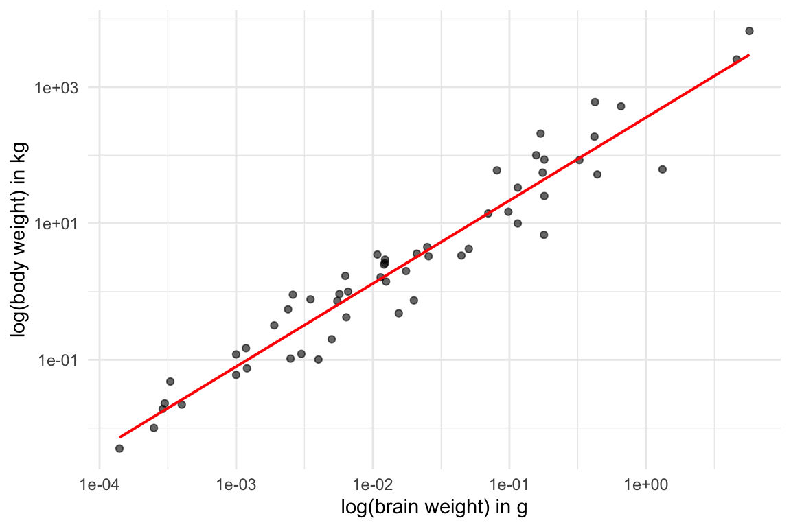
- It appears there may also be a negative, logarithmic relationship (albeit weaker) between the size of mammalian brains and how much they sleep - cool!
ggplot(msleep, aes(x=brainwt, y=sleep_total)) +
    geom_point(alpha=0.6) +
    scale_x_log10() +
    scale_y_log10() +
    stat_smooth(method='lm', col='red', se=F, size=0.7) +
    labs(x='log(brain weight) in g', y='log(total sleep time) in hours') +
    theme_minimal()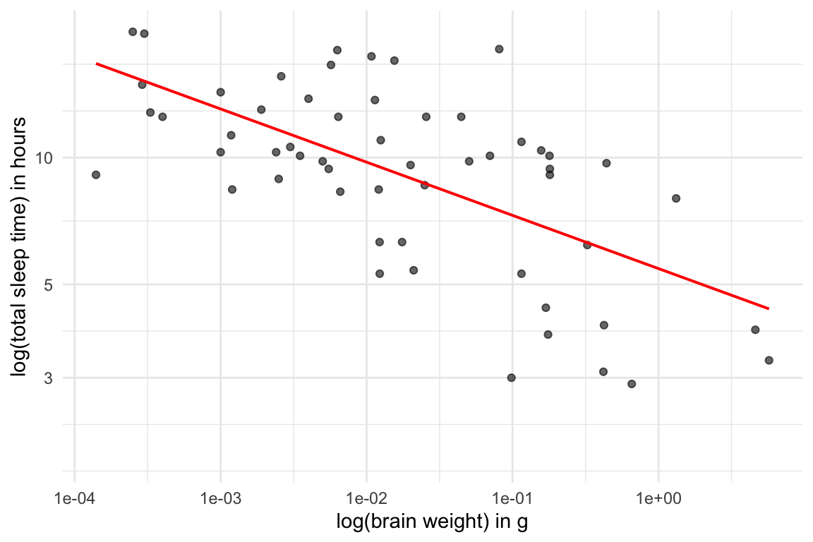
- Wow, there’s a lot of variation in how much different mammals sleep - cool!
ggplot(msleep, aes(x=sleep_total)) +
    geom_histogram() +
    labs(x     = 'Total sleep time in hours',
         title = 'Histogram of total sleep time') +
    theme_minimal()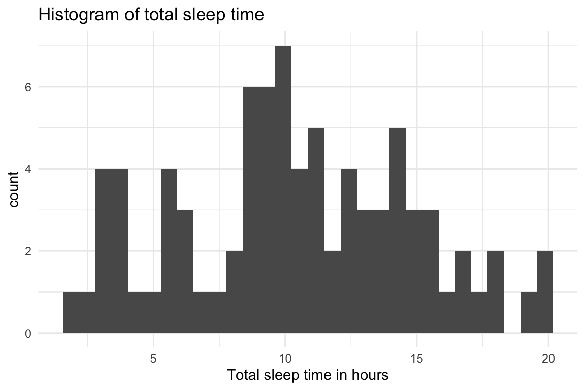
Page sources:
Some content on this page has been modified from other courses, including:
- Data Analysis and Visualization in R for Ecologists, by François Michonneau & Auriel Fournier. Zenodo: http://doi.org/10.5281/zenodo.3264888
George Washington University | School of Engineering & Applied Science
Dr. John Paul Helveston | jph@gwu.edu | Mondays | 6:10–8:40 PM | Phillips Hall 108 | |
This work is licensed under a Creative Commons Attribution 4.0 International License.
See the licensing page for more details about copyright information.
Content 2019 John Paul Helveston