Learning Objectives

Be able to manage computational projects for reproducibility, reuse, and collaboration.

Use R tools and conventions to document code and analyses and produce reproducible reports.

Be able to publish, share materials, and collaborate through the web.

Understand why this all matters!

Suggested Readings

R Markdown: The Definitive Guide, by Yihui Xie, J. J. Allaire, and Garrett Grolemund

RMarkdown Cheatsheet

1 Literate programming

Literate programming is a paradigm first introduced by Donald E. Knuth. The idea is simple:

Treat programs as a literature understandable to human beings

The goal is to integrate data analysis (executable code) with textual documentation, linking data, code, and text together in one document. Literate programming can be directly linked to the concept of reproducibility. Basically, for someone to make a legitimate scientific claim, they should at minimum be able to fully reproduce their results from their raw data (and preferrably others should be able to reproduce them as well).

This leads to the idea of having a reproducible workflow - from raw data to published results.

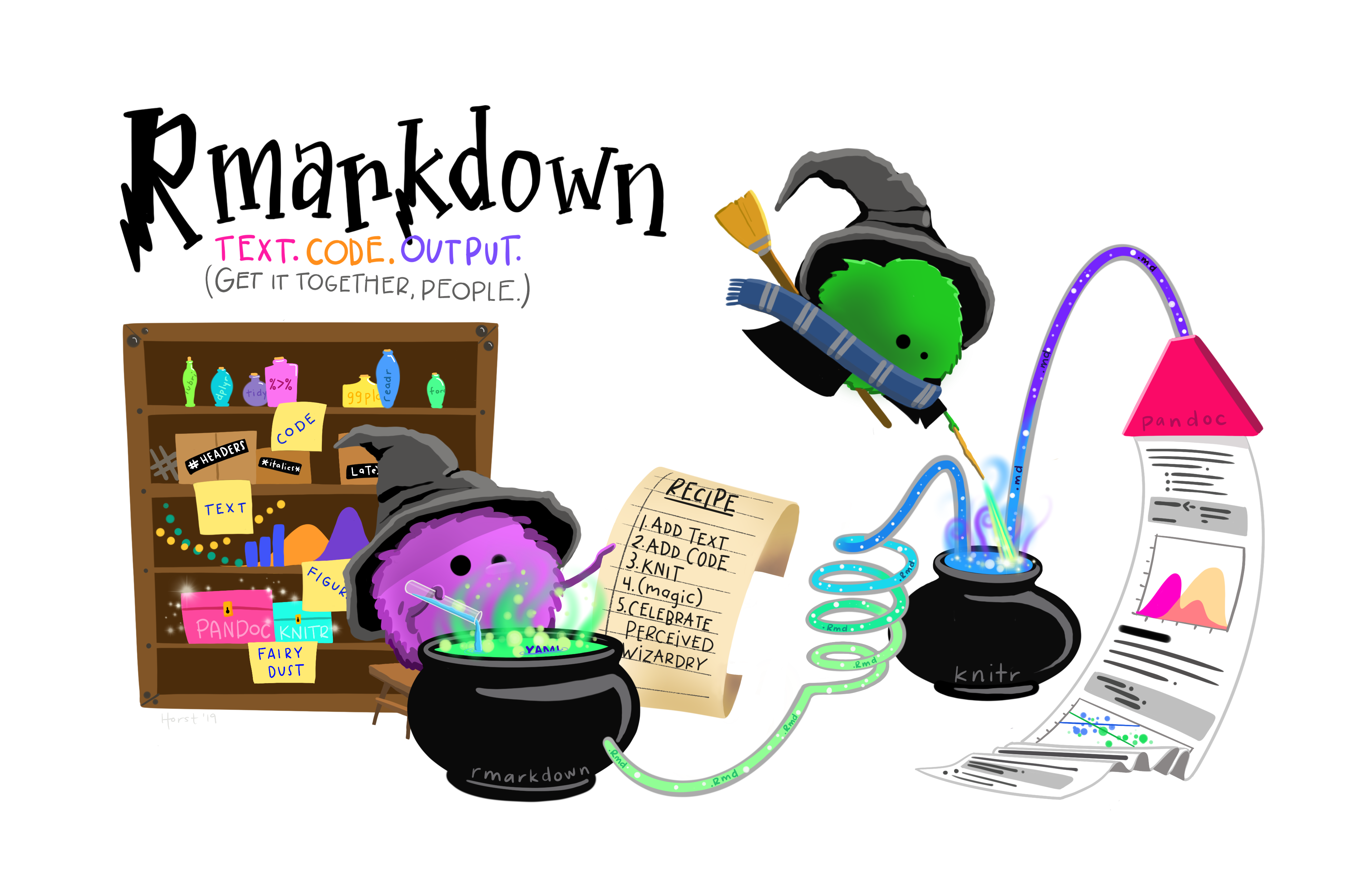
Enter RMarkdown

RMarkdown integrates a documentantion language (markdown) with a programming language (R). This enables authors to craft interactive documents of data, analysis, and results that are easily shareable, particularly through the web.

2 Rmarkdown overview

Watch this 1-min video to get a quick sense of what RMarkdown is:

What is R Markdown? from RStudio, Inc. on Vimeo.

…and watch this 1.5 min video to witness the horrors of not using a reproducible workflow:

3 Elements of RMarkdown

[Art by Allison Horst]

3.1 Markdown

Markdown is a simple, plain text language for converting raw text to HTML for the web (and other outputs, like pdfs). Some of its attributes include:

It has a very small syntax (html links, tables, images, headers, italic / bold font, and a few other things).
It is both easy-to-read and easy-to-write.
It is clean and legible across multiple platforms (including mobile phones).
All formatting is handled automatically through a browser.
Supports raw html as well.

3.2 Code

Code “chunks” are defined through special notation and are executed in sequence throughout the document (just like an .R script). You can mix code directly in with markdown (e.g. “Here’s some simple math in R: 2 + 2 produces 4”) or in separate chunks before or after markdown text. This enables you to write English language text in markdown to explain something, and then immediately follow it up with code to illustrate or demonstrate it.

RMarkdown currently supports a number of different Language Engines through the knitr package, including:

R (default)
Python
SQL
Bash
Rcpp
Stan
JavaScript
CSS

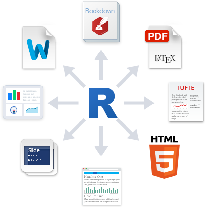
3.3 Outputs

The knitr package enables you to “knit” together the markdown text and R code into a variety of output formats. The default format is an html document for reading through an internet browser and sharing results across the web. Check out the RMarkdown Gallery for some examples. Other formats include:

3.4 Publish to the web

Once you’ve written up your RMarkdown document, you can publish it to the web for free using RPubs: http://rpubs.com/

Watch this quick demo of how to publish your markdown file to the web using RPubs:

4 Elements of a `.Rmd` document

4.1 The YAML header

The yaml header contains metadata about the document - most importantly the output. Different settings can be set within different outputs. Here we’ll be focusing on on the html_document output.

It is contained between these separators at the top of the file.

---

---

Markdown was originally designed for HTML output, so it may not be surprising that the HTML format has the richest features among all output formats. To create an HTML document from R Markdown, you specify the html_document output format in the YAML metadata of your document:

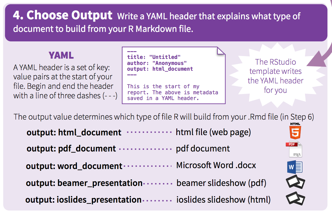
At a bare minimum, your yaml should include a title and output format. Here I’ve also included my name as the author, and the date:

---
title: "This is a demo"
author: "John Helveston"
date: "11/18/2019"
output: html_document
---

This will produce an html page that looks like this:

4.2 Markdown basics

The text in an R Markdown document is written with the Markdown syntax.

Check out this 60-second markdown reference guide to get the basics

If you’re not sure how to make something in markdown, you can try it out first with this handy markdown demo site.

Here’s some of the most-used markdown syntax:

Type this…	…to get this
`normal text`	normal text
`italic text`	italic text
`bold text`	bold text
`*bold italic text*`	*bold italic text*
`superscript^2^`	superscript²
`~~strikethrough~~`	~~strikethrough~~
`code text`	`code text`

For headers, use the # symbol:

# Header 1
## Header 2
### Header 3
#### Header 4
##### Header 5
###### Header 6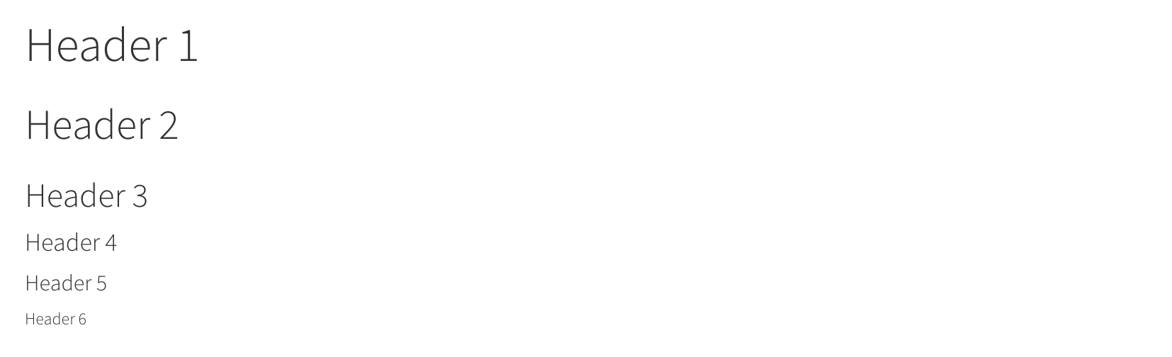

To make a bullet list, use the - symbol:

- first item
- second item
- third item

first item
second item
third item

To make a numbered list, use numbers with a period:

1. first item
2. second item
3. third item

first item
second item
third item

To make a url link to another site, use brackets with parentheses:

[Download R](http://www.r-project.org/)

Download R

To make a basic table, use the | symbol to break up columns, and make a header row by adding -------- underneath the header row:

Table Header  | Second Header
------------- | -------------
Cell 1, 1     | Cell 2, 1
Cell 1, 2     | Cell 2, 2

Table Header	Second Header
Cell 1, 1	Cell 2, 1
Cell 1, 2	Cell 2, 2

Check out this handy online table converter

4.3 Inline R code

You can embed R code directly in a markdown sentence. For example, if you had already created an object x…

x <- 10

…you could use x in a sentence by typing a ` followed by r then any R code you want:

The value of parameter `x` is `r x`, and `2*x` is `r 2*x`

The value of parameter x is 10, and 2*x is 20

Wow - that’s pretty cool!

4.4 R Code chunks

Code chunks are blocks of R code that are executed when you compile the .Rmd document. The output of the code is inserted into the RMarkdown document. Chunks can be used as a means to render R output into documents or to simply display code for illustration (e.g. with option eval=FALSE).

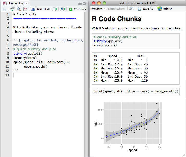
Here’s an example of a .Rmd file with a code chunk on the left and the rendered output on the right:

You can quickly insert an R code chunk with:

The keyboard shortcut Ctrl + Alt + I (OS X: Cmd + Option + I)
The Add Chunk command in the RStudio toolbar
By typing the chunk delimiters ```{r} and ```.

4.4.1 Chunk notation

In between the chunk delimiters ```{r} and ```, you can write R code:

```{r chunk-name}
cat('hello world!')
```

The above R chunk renders as:

## hello world!

You don’t have to name the chunks, but it’s a good practice (like commenting your code). In the above chunk, the name of the chunk is “chunk-name”.

4.4.2 Chunk options

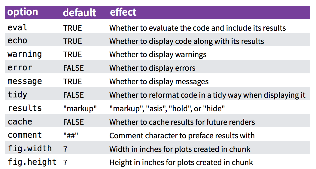
There are lots of options for customizing how markdown chunks appear. By default, code chunks print code + output:

cat('hello world!')

## hello world!

But you can change this by inserting options immediately after the r in the header ```{r} and separate them with commas. For example, if you just want to display the code but don’t want it to actually run, you can add eval=FALSE:

```{r, eval=FALSE}
cat('hello world!')
```

If you only want to print the output (i.e. run the code, but don’t show the code itself), use echo=FALSE:

```{r, echo=FALSE}
cat('hello world!')
```

Finally, if you want to run the code in the background but you don’t want anything to print, use include=FALSE:

```{r, include=FALSE}
cat('hello world!')
```

There are loads of other options for controlling how R chunks behave - here is a list of some (for more details see http://yihui.name/knitr/):

4.5 Plots

By default, figures produced by R code will be placed immediately after the code chunk they were generated from. Here’s an example using ggplot2 to plot the relationship between a couple of variables:

```{r, message=FALSE, fig.height=4, fig.width=6}
library(ggplot2)
library(gapminder)
ggplot(gapminder) +
    geom_point(aes(x = gdpPercap, y = lifeExp, color = continent), size=0.8) +
    theme_minimal()
```

library(ggplot2)
library(gapminder)
ggplot(gapminder) +
    geom_point(aes(x = gdpPercap, y = lifeExp, color = continent), size=0.8) +
    theme_minimal()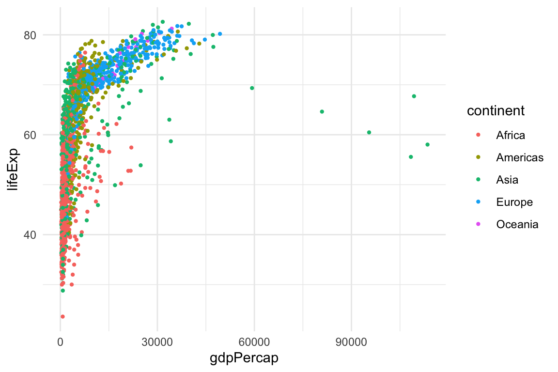

You can adjust the dimensions of plots using fig.height & fig.width inside the chunk settings. For example, in the above plot the setting are {r, fig.height=4, fig.width=6}.

5 Tips

5.1 Knitting to other output formats

As previously mentioned, the default output format for RMarkdown documents is html, but you can change this by adjusting the YAML output. For example, if I wanted to create a pdf document instead, I could use pdf_document in the YAML:

---
title: "This is a demo"
author: "John Helveston"
date: "11/18/2019"
output: pdf_document
---

5.2 Convert a data frame to a table

If you have a table already organized as a data frame in R, rather than painstakingly type the content into a typical markdown table, you can just use the kable() function to directly convert it. Here’s an example using the beatles data frame from the earlier lesson on data frames:

beatles <- data.frame(
    firstName   = c("John", "Paul", "Ringo", "George"),
    lastName    = c("Lennon", "McCartney", "Starr", "Harrison"),
    instrument  = c("guitar", "bass", "drums", "guitar"),
    yearOfBirth = c(1940, 1942, 1940, 1943),
    deceased    = c(TRUE, FALSE, FALSE, TRUE)
)
kable(beatles)

firstName	lastName	instrument	yearOfBirth	deceased
John	Lennon	guitar	1940	TRUE
Paul	McCartney	bass	1942	FALSE
Ringo	Starr	drums	1940	FALSE
George	Harrison	guitar	1943	TRUE

5.3 Inserting a Python code chunk

One of the most impressive things about RMarkdown code chunks is that the code itself doesn’t have to be R code. For example, if you want to use Python code instead, just change {r} to {python} in the code chunk:

'In Python, you can concatenate strings' + ' like this!'

## 'In Python, you can concatenate strings like this!'

6 Additional Resources

Page sources:

Some content on this page has been modified from other courses, including:

R for Reproducible Research, by Anna Krystalli

EMSE 6574, Sec. 11: Programming for Analytics (Fall 2019)
George Washington University | School of Engineering & Applied Science
Dr. John Paul Helveston | jph@gwu.edu | Mondays | 6:10–8:40 PM | Phillips Hall 108 | |
This work is licensed under a Creative Commons Attribution 4.0 International License.
See the licensing page for more details about copyright information.
Content 2019 John Paul Helveston

Data Analysis 4 - Communicating Information

Learning Objectives

Suggested Readings