Programming Basics
1 Functions
You can do a lot with the basic operators like +,
-, and *, but to do more advanced calculations
you’re going to need to start using functions.1
R has a lot of very useful built-in functions. Suppose I wanted to take the square root of 225. The usual notation for this is \(\sqrt{25}=5\), though sometimes you’ll also see it written like this \(25^{0.5} = 5\). This second way of writing it is kind of useful to “remind” you of the mathematical fact that “square root of \(x\)” is actually the same as “raising \(x\) to the power of 0.5”. And since we already know how to raise things to powers in R, we could do this:
225 ^ 0.5## [1] 15However, we could also compute this using R’s built-in square root
function sqrt():
sqrt(225)## [1] 15Not sure what a particular function does? You can ask R for help by
typing ? and then the function name, and R will return
documentation on the function. For example, ?sqrt() will
return information about the sqrt() function.
1.1 Some common functions
| Function | Description | Example |
|---|---|---|
exp() |
Exponential | exp(0) returns 1 |
sqrt() |
Square root | sqrt(64) returns 8 |
log(x) |
Natural log of x |
log(1) returns 0 |
factorial() |
Factorial | factorial(5) returns 120 |
round(x, digits=0) |
Round x to the digits decimal place |
round(3.1415, digits=2) returns 3.14 |
abs(x) |
Absolute value of x |
abs(-42) returns 42 |
1.2 Combining functions
In the same way that R allows us to put multiple operations together
into a longer command (like 1 + 2 * 4 for instance), it
also lets us put functions together and even combine functions with
operators if we so desire. For example, the following is a perfectly
legitimate command:
sqrt(1 + abs(-8))## [1] 3When R executes this command, starts out by calculating the value of
abs(-8), which produces an intermediate value of
8. The command then simplifies to sqrt(1 + 8).
To solve the square root2 it first needs to add 1 + 8 to
get 9, at which point it evaluates sqrt(9),
and so it finally outputs a value of 3.
2 Arguments
When we use a function to do something, we generally refer to this as calling the function. The values that we type into the function are referred to as the arguments of that function. Some functions can have more than one argument.
2.1 Multiple arguments
Some functions have more than one argument. For example, the
round() function can be used to round some value to the
nearest whole number. For example, I could type this:
round(3.1415)## [1] 3Pretty straightforward. However, suppose I only wanted to round it to
two decimal places: that is, I want to get 3.14 as the
output. To do this, you can input a second argument that specifies the
number of decimal places that you want to round the number to. To get
3.14, I would type this:
round(3.14165, 2)## [1] 3.142.2 Argument names
In this simple example, it’s not too hard to remember which argument
comes first and which one comes second, but it starts to get very
difficult once you start using complicated functions that have lots of
arguments. Fortunately, most R functions use argument
names to make your life a little easier. For the
round() function, for example, the number that needs to be
rounded is specified using the x argument, and the number
of decimal points that you want it rounded to is specified using the
digits argument:
round(x = 3.1415, digits = 2)## [1] 3.142.3 Default values
Notice that the first time I called the round() function
I didn’t actually specify the digits argument at all, and
yet R somehow knew that this meant it should round to the nearest whole
number. How did that happen? The answer is that the digits
argument has a default value of 0, meaning
that if you decide not to specify a value for digits then R
will act as if you had typed digits = 0. This is quite
handy: most of the time when you want to round a number you want to
round it to the nearest whole number, and it would be pretty
annoying to have to specify the digits argument every
single time. On the other hand, sometimes you actually do want to round
to something other than the nearest whole number, and it would be even
more annoying if R didn’t allow this! Thus, by having
digits = 0 as the default value, we get the best of both
worlds.
Finally, not all functions have (or require) arguments:
date()## [1] "Wed Apr 12 17:32:06 2023"3 Objects
In R, all “assignments” have this form:
objectName <- valuewhere the arrow, <-, means “assign value
to objectName”.
The operator <- is a pain to type, so RStudio has a
keyboard shortcut: Alt + - (the minus sign). RStudio offers many other
handy keyboard
shortcuts. Also, Alt+Shift+K brings up a keyboard shortcut reference
card.
To practice, try assigning 2 to x:
x <- 2Now type x again - notice that it returns the value
assigned to it!
x## [1] 2If you overwrite an object with a different value, R will “forget” the previous assigned value and only keep the new assignment:
x## [1] 2x <- 42
x## [1] 42A note on formatting: Always surround
<- with spaces! Otherwise your code can be confusing.
For example, if you typed x<-2 (no spaces), it’s not
clear if you meant x <- 2 or x < -2. The
first one assigns 2 to x, but the second one
compares whether x is less than -2.
3.1 Object names
You can choose almost any name you like for an object, as long as the
name does not begin with a number or a special character like
+, -, *, /,
^, !, @, or &.
You will be wise to adopt a convention for
demarcating words in names. Here are a few:
snake_case_is_one_choiceother.people.use.periodscamelCaseIsAlsoGood
Make another assignment:
this_is_a_really_long_name <- 2.5To inspect this, try out RStudio’s completion facility: type the first few characters, press TAB - voila! RStudio auto-completes the long name for you :)
R is case sensitive. To understand what this means, try this:
cases_matter <- 2^2
Cases_matter <- 2^3
Let’s try to inspect:
cases_matter## [1] 4Cases_matter## [1] 8Although the two objects look similar, one has a capital “C”, and R stores that as a different object.
In general, type carefully. Typos matter. Case matters. Get better at typing.
3.2 The workspace
Look at your workspace in the upper right pane. The workspace is where user-defined objects accumulate. You can also get a listing of these objects with commands:
objects()## [1] "cases_matter" "Cases_matter"
## [3] "this_is_a_really_long_name" "x"ls()## [1] "cases_matter" "Cases_matter"
## [3] "this_is_a_really_long_name" "x"If you want to remove the object named x, you can do
this
rm(x)To remove everything, use this:
rm(list = ls())or click the broom in RStudio’s Environment pane.
4 Data types
Every programming language has the ability to store data of different types. R recognizes several important basic data types (there are 6 total, but these 4 are all we’ll ever use):
| Type | Description | Example |
|---|---|---|
| numeric | Numbers | 3.14, 42, 1.61803398875 |
| integer | A number with no decimal | 1L, 7L |
| character | Text data, a.k.a. “strings” | "this is a string", "3.14" |
| logical | Used for comparing objects | TRUE, FALSE |
To assess the type of any variable, R has two different functions:
class()tells us the high level object typetypeof()tells us the low level object type
We’ll use these to explore each data type.
4.1 Numeric types
Numbers in R are of the numeric data type, and it is the
default computational type. There are two types of numeric data types:
integers and floats. The difference is
floats have decimals and integers don’t. At the lower level, floats have
the type “double” while integers have the type
“integer”.
By default, R assumes all numbers are floats, even if it looks like an integer:
class(3.14)## [1] "numeric"class(3)## [1] "numeric"typeof(3.14)## [1] "double"typeof(3)## [1] "double"The fact that 3 is not an integer can be confirmed with
the is.integer()function:
is.integer(3)## [1] FALSETo make a number an integer, you have to either add an L
to the end, or use the as.integer() function to coerce it
into an integer type:
typeof(3L)## [1] "integer"typeof(as.integer(3))## [1] "integer"Note that you can have a decimal of 0 but the data types
can be different:
typeof(7)## [1] "double"typeof(7.0)## [1] "double"typeof(7L)## [1] "integer"4.2 Character types
A character object is used to represent string values in R. Anything
put between single quotes ('') or double quotes
("") will be stored as a character. For example:
s <- '3.14'
class(s)
## [1] "character"Notice that even though the value assigned to s is a
number, it is stored as a character because the number is surrounded by
quotes. If you mistakenly thought it was stored as a number, R will
gladly return an error when you try to do a numerical operation with
it:
s + 7## Error in s + 7: non-numeric argument to binary operatorWe can also convert objects into character values with the
as.character() function:
a_number <- 3.14
class(a_number)
## [1] "numeric"a_string <- as.character(a_number)
class(a_string)## [1] "character"We will go into much more detail about character data later on in Week 6
4.3 Logical types
A logical value is usually created when comparing variables. For example, let’s compare whether one value is greater than another:
x <- 1
y <- 2
z <- x > y # Is x greater than y?
z
## [1] FALSEThe object z now stores the value (FALSE)
that resulted from comparing x and y.
To compare whether two values are equal, you have to type the
= sign twice:
x == y## [1] FALSEHere I am asking, “is x equal to y”? In
this case, the answer is FALSE.
We will go into more detail about comparing values in R later on in Week 4
4.4 Special values
In addition to the four main data types mentioned, there are a few
additional “special” types: Inf, NaN,
NA and NULL.
Infinity: Inf corresponds to a value
that is infinitely large. You can also have -Inf. The
easiest way to get Inf is to divide a positive number by
0:
1/0## [1] InfNot a Number: NaN is short for “not a
number”, and it’s basically a reserved keyword that means “there isn’t a
mathematically defined number for this.” For example:
0/0## [1] NaNNot available: NA indicates that the
value that is “supposed” to be stored here is missing. We’ll see these
much more when we start getting into data structures like vector,
matrices, and data frames.
No value: NULL asserts that the
variable genuinely has no value whatsoever, or does not even exist.
4.5 Coercing data types
In general, you can force an object into a different type using
as.something(), replacing “something” with a
data type:
as.numeric(3.1415)## [1] 3.1415as.integer(3.1415)## [1] 3as.character(3.1415)## [1] "3.1415"as.logical(3.1415)## [1] TRUENote that as.logical() returns TRUE for any
numeric value other than 0, for which it returns
FALSE.
If you try to coerce a string into a number, R will return
NA:
as.numeric('foo')## Warning: NAs introduced by coercion## [1] NAIf you want to force a float number (i.e. one with decimals) into an
integer value, but you don’t want to change the actual type to
an integer type, use round(), ceiling(), or
floor(). This will turn the number into an integer in
value, but will still technically be float types. Note that
these functions produce different outcomes.
round(3.1415) # Typical rounding## [1] 3ceiling(3.1415) # Rounds *up* to nearest integer## [1] 4floor(3.1415) # Rounds *down* to nearest integer## [1] 35 Packages
When you start R, it only loads the “Base R” functions. But there are thousands and thousands of additional functions stored in packages.
There is a critical distinction that you need to understand, which is the difference between having a package installed on your computer, and having a package loaded in an R session. You only need to install a package to your computer once, but you will need to load it whenever you want to use it in any one R session. This relationship is illustrated in the image below:
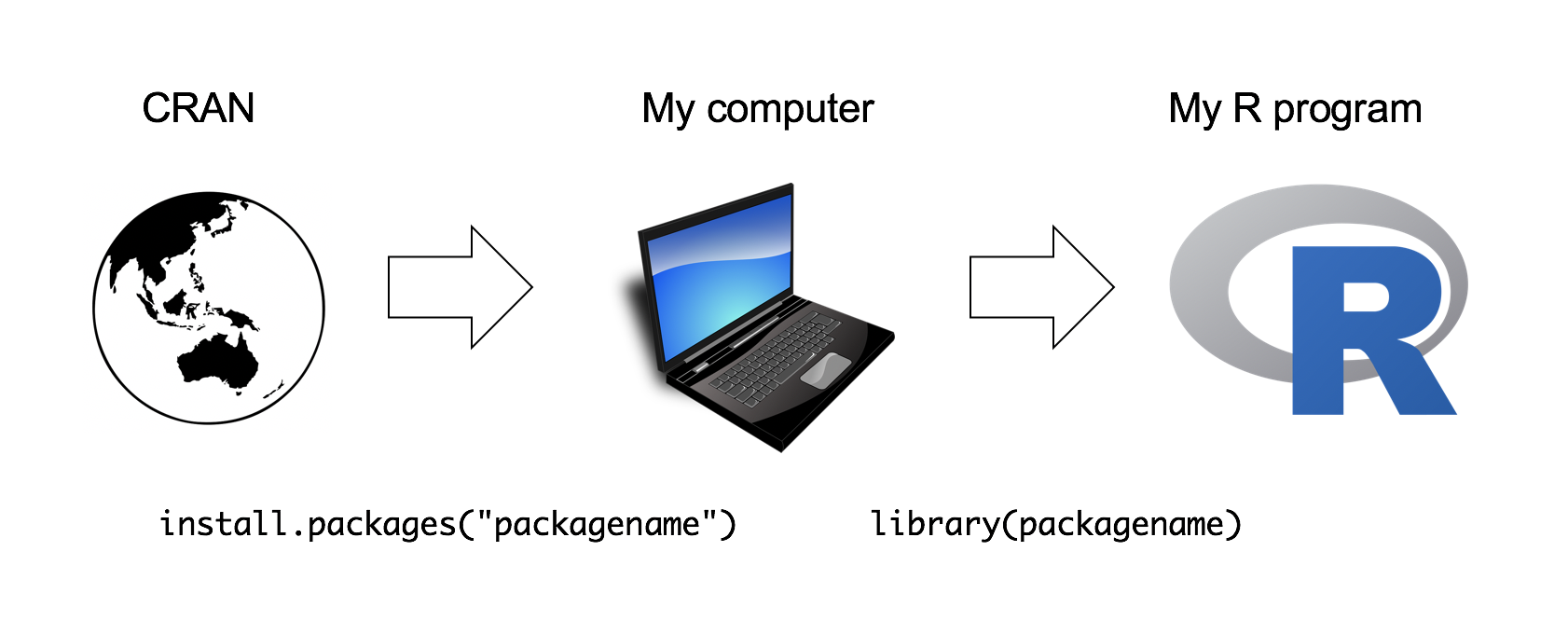
When installing a package, you must put the package name in quotes:
install.packages("packagename") # This works
install.packages(packagename)   # This doesn't work
When loading a package in an R session, you don’t have to use quotes (but you can if you want):
library("packagename") # This works
library(packagename)   # This also works
As an example, try installing the Wikifacts package, by Keith McNulty:
install.packages("wikifacts") # Remember - you only have to do this once!Now that you have the package installed on your computer, try loading
it using library(wikifacts), then trying using some of it’s
functions:
library(wikifacts) # Load the librarywiki_randomfact()## [1] "Did you know that on January 23 in 1565 – The Deccan sultanates defeated the Vijayanagara Empire at the Battle of Talikota in present-day Karnataka, ending the last great Hindu kingdom in southern India. (Courtesy of Wikipedia)"wiki_didyouknow()## [1] "Did you know that the Tokushima-Kōchi at-large district elected its first representative to the House of Councillors this month? (Courtesy of Wikipedia)"In case you’re wondering, the only thing this package does is generate messages containing random facts from Wikipedia.
6 Tips
6.1 Check if a number is an integer
If you use the is.integer() function to check if a
number that looks like an integer, you might get a
surprising result:
is.integer(7)## [1] FALSEThis is because the default numeric type is a float. The safer way to check if a number is an integer in value is to compare it against itself as an integer:
7 == as.integer(7)## [1] TRUEIn your assignments, use this method to check if something is an integer!
Page sources:
Some content on this page has been modified from other courses, including:
- Danielle Navarro’s website “R for Psychological Science”
- Jenny Bryan’s STAT 545 Course
- RStudio primers
- Xiao Ping Song’s Intro2R crash course
Footnotes
Technically speaking, operators are functions in R: the addition operator
+is a convenient way of calling the addition function'+'(). Thus10+20is equivalent to the function call'+'(20, 30). Not surprisingly, no-one ever uses this version.↩︎R does support complex numbers, but unless you explicitly specify that you want them it assumes all calculations must be real valued. By default, the square root of a negative number is treated as undefined:
sqrt(-9)will produceNaN(not a number) as its output. To get complex numbers, you would typesqrt(-9+0i)and R would now return0+3i.↩︎
George Washington University | School of Engineering & Applied Science
Dr. John Paul Helveston | jph@gwu.edu | Mondays | 6:10–8:40 PM | Phillips Hall 108 | |
This work is licensed under a Creative Commons Attribution 4.0 International License.
See the licensing page for more details about copyright information.
Content 2019 John Paul Helveston